|
|
| The transputer based
navigation system - an example of testing embedded systems _____________________________________________________________________ |
| INMOS 72-TCH-002 |
This note covers the implementation of the Navigation System outlined in Technical Note 0, ’A transputer based radio-navigation system’.
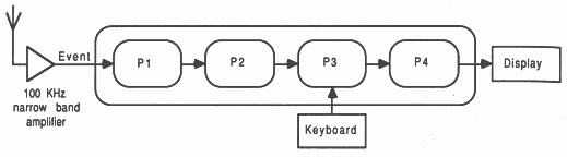
The software described in Technical Note 0 consisted of 4 concurrent processes in a pipeline, as shown in figure 1.
These processes performed the following tasks:
Just as the ’Divide and Conquer’ method eased the design of the software, similarly it allows the software to be tested and debugged without difficulty.
Each process is provided with input data, and is output is checked. Taking the independence of each process into full account allows independent test-data generators to be produced for each, and this is the recommended method if P1 thru P4 are being developed simultaneously by separate teams. However, when one team is developing each in turn, only a single test generator is required; when P1 is correct, its output can be used to test P2 and so on. Note that this latter method does not test the resilience of subsequent processes to incorrect data, while the former method does.
The system does require resilience to incorrect input data, even if P2 to P4 do not and the method of ensuring this is covered later.
Once the code for P1 is written, a test-data generator is required. This software test-data generator replaces the hardware environment that would normally feed the data.
The most convenient way of testing is to ensure that the process accepts correct data first, and then to extend it to correctly reject erroneous data. To generate the correct data, another process is written.
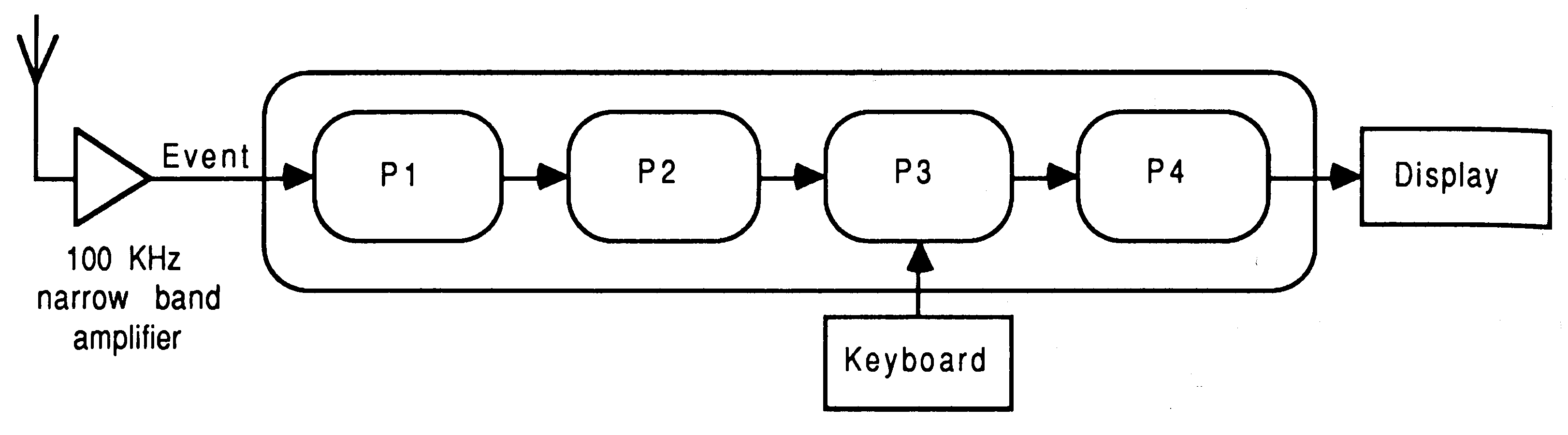
In the case of the navigation system, the input data is the off-air signal from a chain of transmitters. The incorrect data is interference from other chains of transmitters and from random noise. Thus the first test harness consists of a control environment that manages keyboard and screen of the development system, and a process that mimics a chain of transmitters on figure 2.
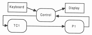
This would be ideal, but when it is wrong, how can an error in the controller, TC1 or P1 be traced? In this case the harness is debugged by first using just TC1 with the control - figure 3.
This allows TC1 and the controller to be interactively tested on-screen; feeding in new parameters and checking the data generated.
The generated data consists of a stream of numbers, being the timestamp associated with each zero-crossing of the carrier waveform. The carrier is in groups of bursts, as shown below in figure 4.
The parameters fed to TC1 are Delay 1, Delay 2, Delay 3 and the Group Repetition Interval (GRI). In order to facilitate testing, the development system screen was divided into 3 windows, and a menu created. The menu controlled the test environment, displayed in the first window, and the user inputs to the navigation system; i.e. its front panel controls were displayed in the second window. The third window displayed the results from the system, and so represented the front panel display of the navigation system.
Once the harness was debugged, the configuration of figure 2 was used to debug and tune P1. ’Tune’ should be stressed because there were many constant parameters to each process that determined hour, selective/tolerant it should be, there being a trade-off, of course, between tolerance, accuracy, and resilience, defined here as the ability to continue functioning in the face of adverse conditions - for example in the case of intermittent lack of input data.
The job of P1 is to monitor each supposed carrier transition, validate it as being the correct frequency, and of adequate duration, then pass on its initial timestamp and mean phase to P2.
As the incoming carrier has a frequency of 100KHz, consecutive events should occur at 10 microsecond intervals. Thus P1 checks that the interval is within limits (currently set to 9 to 11, as the system implemented differs from Technical Note 0 in feeding the signal direct to the transputer’s event pin, giving 1 microsecond resolution on the internal timer, rather than via an external timer).
It then counts a preset number of validated transitions, and if it reaches the threshold, currently set to 10, it accepts the signal as being genuine and passes on to P2 a timestamp-pair, consisting of the timer value of the first transition and the sum of the 10 phase values. This latter figure allows the effective resolution to be increased by a venire effect between the RF carrier and the transputer crystal over the whole burst, or group of bursts.
P1 was tested and tuned until the bursts of signal at its input were correctly presented to P2; or at this stage, displayed on the screen.
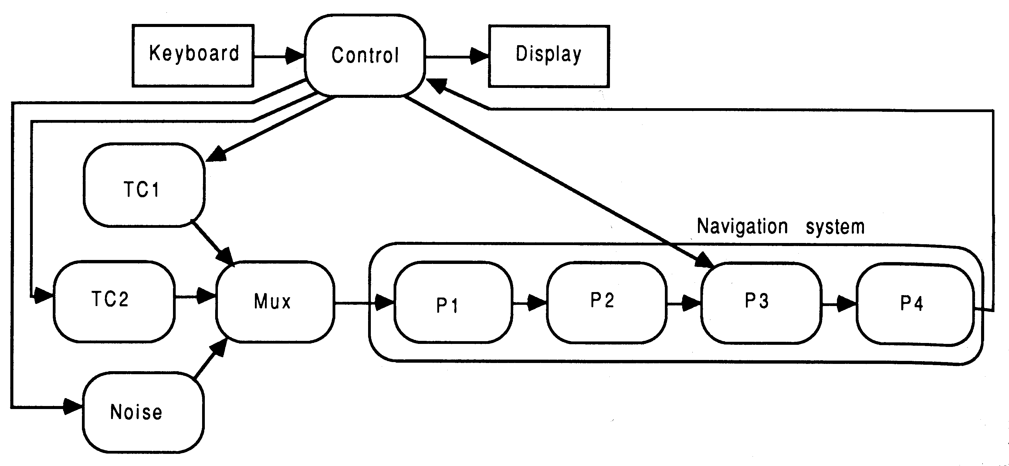
One of the functions of P1 is to discriminate against noise, so to test this the ability to inject noise was required. This was achieved by expanding the test harness to generate noise. This meant two new processes, one to generate timestamps representing noise, and the other to multiplex the data sources, sorting timestamps into the correct order - see figure 5.
Although not fully rigorous, the noise type chosen was bursts of carrier described by their carrier period, the number of cycles in a burst, and the burst repetition rate, so each of these became parameters in the menu window.
The multiplexer simply performed an input as necessary on each stream to ensure it had access to the next data item on each stream. It then selected the earliest timestamp, and passed it to P1, replenishing itself from the stream chosen. Notice that no analogue level was considered - the high gain limiting amplifier was considered to have made all inputs full strength. However, time distortion was added; if two timestamps were too close (currently 4 microseconds), they would both be deleted, and replaced with a single transition at the mean of the two: - again, not rigorous, but implementing some approximation to real interference.
Once P1 had been proven to the harness, P2 was added. The function of P2 is to monitor the carrier bursts it receives, and validate them into correct groups for master or slave transmitters. A slave transmitter generates eight bursts at one millisecond intervals, and a master 9 bursts, spaced as if the group were ten bursts with the ninth omitted.
It can be seen that there is massive data reduction down the pipeline. P1 expects an input every 10 μs, P2 every 1 ms, P3 approximately every tenth of a second; these are peak rates - the duty cycle is very low. As a result of the data reduction, more thorough testing is feasible as the later processes are added, as the volume of data on the screen reduces.
This implementation uses visual checking; it would be perfectly possible to correlate output and input in another process and report only statistics. This method was rejected because the final navigation system generates only two outputs - LATitude and LONGitude; the visual approach is entirely satisfactory.
To validate bursts, P2 checks that they are at one millisecond intervals, plus/minus a tolerance, currently set to 5 microseconds. Again, the benefit of the harness is seen in allowing the system to be tuned. It then counts validated bursts. The subtle part is how to optimally detect master transmitters, as the process only runs when triggered by an input, so if the final pulse never comes, it is a slave, but the process does not run to report this.
The solution is simple, once found. It is important not to waste CPU time, so to deschedule the process and wait on a timer for 2+ milliseconds would be a problem, but is the easiest to implement. However, there is no problem of latency in the pipeline - it does not matter if the screen display runs milliseconds after the input all the data inputs were timestamped on reception, so accuracy is maintained. Thus no output is generated until the next input burst, when the decision is made whether it is the ninth burst of the group (i.e. it was a master) or the first of an independent group (it was a slave).
Part of the validation task performed by P2 is to reject groups that have been corrupted by overlapping between two transmitter chains.
If the bursts collide directly, P7 will reject them. However, because of the low duty cycle it is possible that they may interleave. In this case the current implementation of P2 will lock onto the group starting first, and ignore the interleaved bursts as each is ’too early’ in its opinion. This is not the optimum solution, as the second group may be the desired one. However, P2 is ignorant of this, it being decided in P3, and to track two groups simultaneously adds unnecessary complication. It could be done, however, if the LORAN time domain became too cluttered in some areas.
All these functions can be tested by adding a second transmitter chain (TC2) to the environment. Experiments can then be performed with the two chains with very close repetition intervals. Again, due to the data reduction, this testing can be extended greatly after P3 is written.
The final test harness is shown in figure 6, used first with P1 and P2, then P1 to P3, then P1 to P4.
P3 is the most complex and thus requires most testing and tuning. Its task is twofold - i.e. it has two modes of operation. First it must identify and lock onto the correct transmitter chain, then it must monitor it, even though a large percentage of its transmissions may have been lost due to noise or other transmitters interfering.
The first task is performed by capturing a buffer full of detected groups, and then searching the buffer for groups that have the correct repetition interval. The buffer must be large enough to cover at least two frames, in order that spurious internal matches be excluded, and again, the tolerance on the matching requires tuning.
If there is not suitable match, the initialisation phase starts again, and repeats until successful.
Once the timestamps of the required transmitter chain are found, the process predicts when the next will be, and validates against that. If a timestamp is missed, a new prediction is made, and the omission noted. After a set number of omissions in a row (currently 5), the system admits a synchronisation failure and reverts to initialisation mode..
Thus the ’locking’ criteria can be tuned against the ’unlocked’ criteria. As set at present, there will be the occasional false lock, which will then find no valid frames and re-initialise. Final tuning of this will be done in the real world, when the level of noise etc. is real, not simulated.
At each successful frame, P3 passes on the delay values to P4, which performs the mathematics and displays the ship’s position.
Two improvements were made to P3, P4 to maximise the performance of the system.
In P3, allowance was made for errors in frequency between the transmitter crystal and the transputer crystal. Although partly covered by the timing tolerances in P1 to P3 already, because P3 assumes missed signals, and predicts future ones, any error is multiplied by the number of frames covered. Thus while it is instructed to use a particular Group Repetition Interval, it will actually use one extracted off-air, within a tolerance (currently 48 microseconds).
This greatly improved the system noise tolerance.
In P4, rather than update the display every tenth of a second, which is too fast for the human eye, causes excessive least-significant digit fitter, and uses excessive CPU time, the delay signals were validated by collecting them for a period (currently 2 seconds), rejecting fitter-rogues, and then calculating and displaying.
It can be seen that the software harness allowed demonstration of the system, basic debugging, error-handling, performance enhancements, all before an oscilloscope was bought to test the hardware! It will also allow continued testing with real input data, but display via the development system, giving the opportunity for final program tuning in RAM before the ROMs are programmed and the system goes live across the ocean.