|
|
| Performance Maximisation _____________________________________________________________________ |
| Phil Atkin March 1987 |
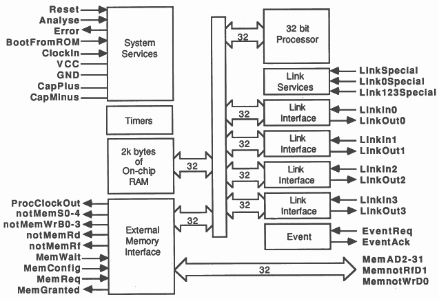
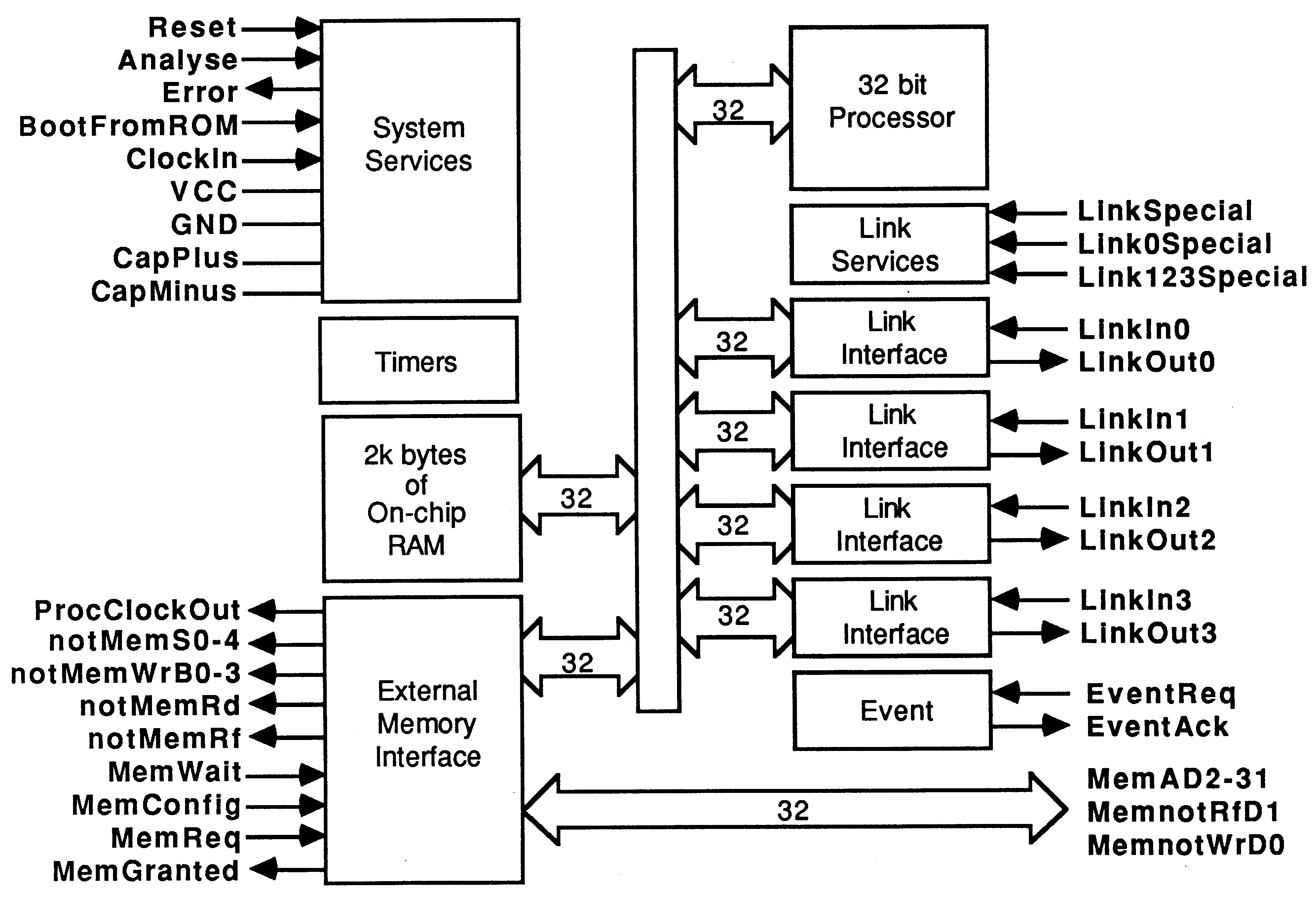
The INMOS transputer family [1] is a family of microcomputers with high-performance processor, memory and communication links on a single chip, Figure 1. The links are used to connect transputers together, and very large concurrent systems can be built from collections of transputers communicating via their links.
The occam programming language [2] was developed by INMOS to address the task of programming extremely concurrent systems. This document will illustrate how best to arrange occam programs in order to maximise the performance of transputer systems, with particular reference to the author’s ray-tracing program [4].
All these performance enhancement techniques have been implemented in the ray tracer, and their use will be illustrated by fragments from this program.
Several topics will be discussed, falling into two main categories - maximising the performance of an individual transputer, and maximising the performance of arrays of transputers.
Note that all occam examples conform to the beta release of the Transputer Development System.
The following sections describe how to maximise the performance of a single transputer. However, all these performance maximisation techniques are highly relevant to maximising the performance of each processor in a multiple transputer system.
To achieve maximum performance from a transputer it is vital that best use is made of on-chip memory. On the B004-4 Transputer Evaluation Board for example [6], the internal memory cycles in 66ns, whereas the off-chip memory cycles in 330ns. This factor of five degradation in memory speed can be reflected in program performance if heavily accessed locations are in off-chip memory.
On-chip memory is better used for data, rather than code. The T414 fetches instructions in 32-bit words, so every code fetch cycle will pull in 4 instructions. Hence code accesses generally occur less frequently than data accesses, and data memory requires higher bandwidth.
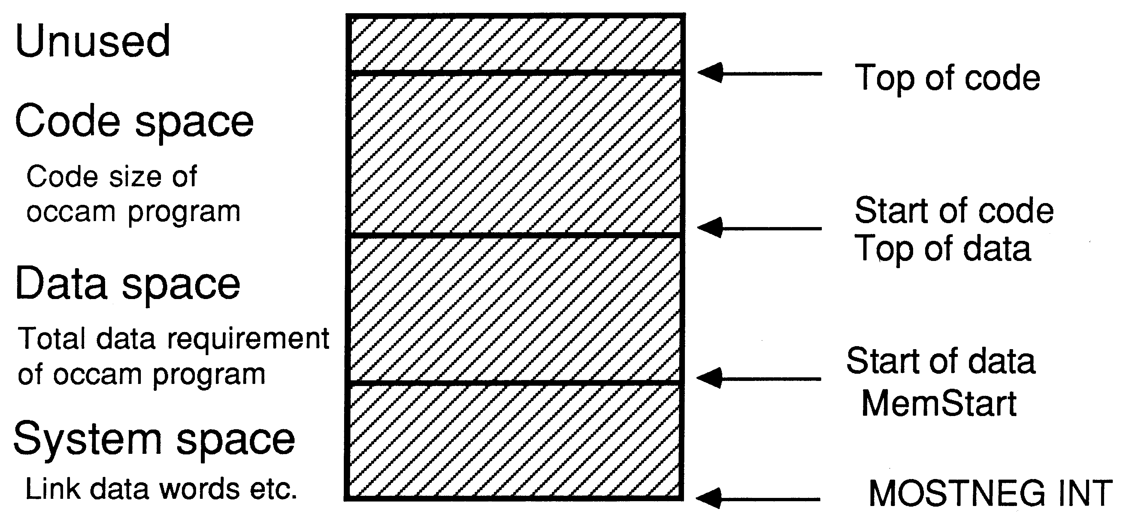
The occam compiler and transputer loader software take advantage of this bandwidth imbalance between data and code memory by trying to place data on-chip (Figure 2). Data space is allocated upwards from the lowest free location in on-chip memory, and code is placed immediately above the highest data location.
This is made possible because all data allocation in occam is static, and after compilation the loader knows exactly the data space requirement of the program. (Static allocation has one major drawback - recursion is not allowed in occam. Handling recursive algorithms in occam is described in Appendix A.)
If a program has a data space requirement of more than 2k bytes (the on-chip memory space of the T414), then some data will be placed in off-chip memory. It is then up to the programmer to arrange his occam program such that the most frequently-used variables are placed on-chip. The following sections will describe how to write occam programs which optimise use of on-chip memory.
On the transputer, variables are accessed relative to a workspace pointer register, Wptr [1]. Each occam process has its own workspace - a procedure call will generate a new workspace for the called procedure, and forking a set of parallel processes will generate a new workspace for each new process.
To maximise performance it is important that variables within the most frequently active workspace areas be in on-chip memory.
The occam compiler places the most recently declared variables in the lowest workspace slots. For example, the following piece of code
INT32 a, b, c :
[2000] INT32 largeVector : SEQ a := 42 b := #DEFACED c := #DEAF SEQ i = 0 FOR 2000 largeVector [i] := 0 |
would result in the following workspace layout
| Variable | Workspace Location |
| a | 2005 |
| b | 2004 |
| c | 2003 |
| largeVector | 2 .. 2002 |
| i | 0 .. 1 (replicators consume 2 workspace slots) |
Note that the replicator variable, is implicitly declared last, and therefore takes up the two lowest workspace slots. However, a, b and c have ended up off-chip, and they will be relatively expensive to access - prefixing instructions are required to access them, and accessing off-chip memory will consume extra processor cycles. If a, b or c are going to be accessed frequently, it is better to declare them after largeVector.
In occam, workspace for called procedures is allocated as a falling stack. Called procedures have their workspace placed at lower addresses than the caller. All vectors are located by the compiler within the workspace of the process in which they are declared. Hence the occam compiler does nothing to improve the performance of this piece of code -
[2000] INT32 largeVector :
INT32 a, b, c : PROC totallyWasteOnChipMemory () [2000] INT32 largeData : SEQ i = 0 FOR 2000 largeData [i] := i : SEQ totallyWasteOnChipMemory () a := 42 b := #DEFACED c := #FADED SEQ i = 0 FOR 2000 largeVector [i] := 0 |
The call of totallyWasteOnChipMemory takes up over 2000 words of low-address memory, consuming all of the on-chip memory.
Calling a procedure with a large workspace requirement results in the caller process having its workspace placed entirely off-chip. A good rule to improve performance is declare all large vectors at the outermost lexical level.
NOTE
Unfortunately this is not good programming practice - declaring items at the scope
within which they are required is more secure, avoiding accidental shared data or
other programming errors. This conflict of good programming style and program
efficiency is a feature of the current compiler implementation, not the occam
language. It is intended that future releases of the occam compiler will allow the
user to specify whether vectors should be compiled located within or outside the
current workspace.
To avoid lengthy access times due to static chaining, these global vectors should be brought into local scope, either by passing them as parameters, or abbreviating them locally to their use.
Using abbreviations to bring large vectors into local scope has a dramatic effect on workspace requirement.
[2000] INT32 largeVector, vectorForPROC :
INT32 a, b, c : PROC totallyWasteOnChipMemory () [2000] INT32 largeData IS vectorForPROC : SEQ i = 0 FOR 2000 largeData [i] := i : SEQ totallyWasteOnChipMemory () a := 42 b := #DEFACED c := #FADED SEQ i = 0 FOR 2000 largeVector [i] := 0 |
This simple change to totallyWasteOnChipMemory has reduced its workspace requirement from over 2000 words to only 3 words (the abbreviation, and 2 words for i), leaving large amounts of on-chip memory free for other processes.
Further use of abbreviations to improve performance is discussed in sections 2.1.5 - 2.1.8.
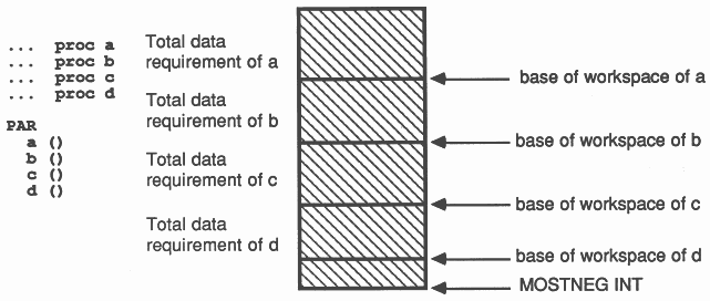
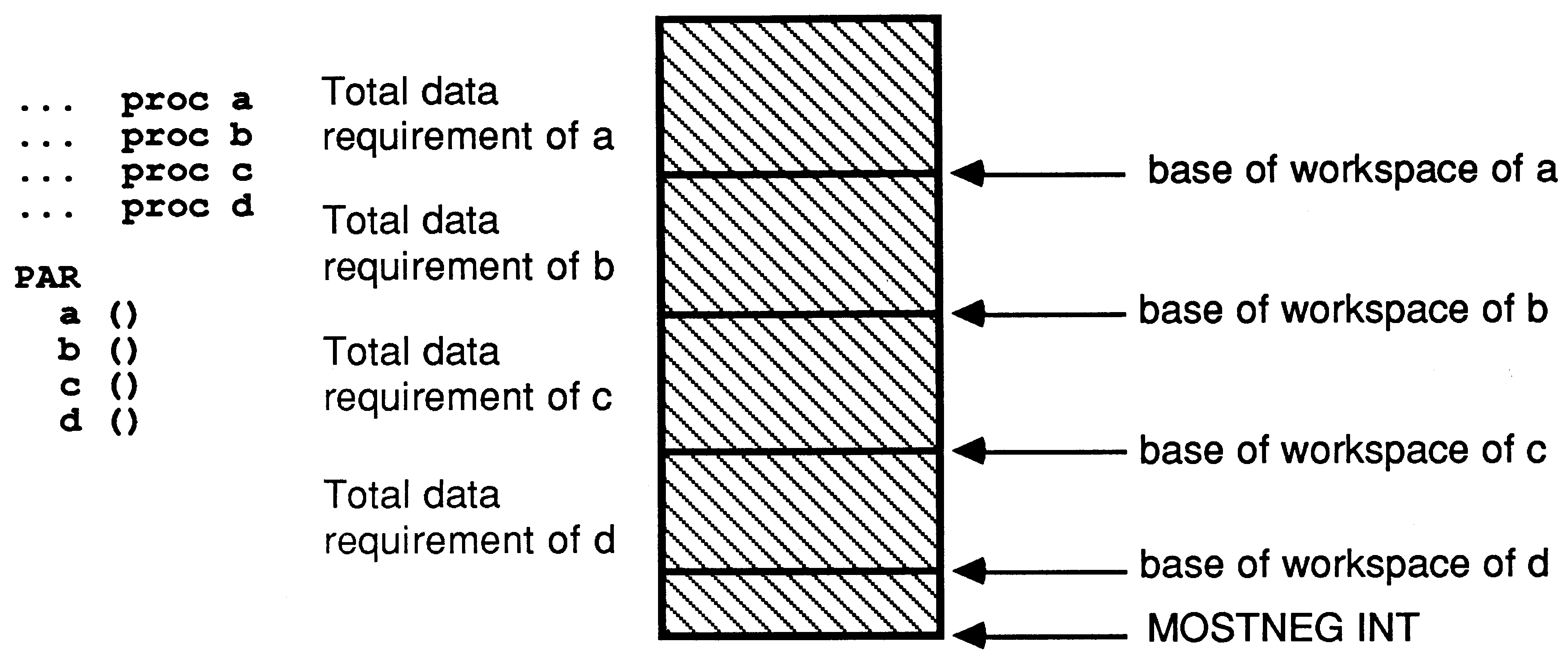
Workspace for parallel processes is allocated below the workspace of the parent. The first member of the PAR list is allocated workspace immediately below the parent, the second immediately below that, etc.
Hence workspace minimisation by global declaration becomes even more important when more than one process is running on the transputer. If, in the example above any of the processes a, b, c or d were consuming large amounts of workspace, then the workspace of the others could be resident off-chip. To ensure minimisation of workspace in a parallel environment, large vectors must be declared outside the scope of the outermost PAR. For example,
PAR
[2000] INT vector : a ( vector ) [2000] INT vector : b ( vector ) [2000] INT vector : c ( vector ) [2000] INT vector : d ( vector ) |
is not sufficient; the large vectors are declared within the scope of the PAR, and will contribute to the workspaces of the individual processes. The program should be
[2000] INT vecA, vecB, vecC, vecD :
PAR a ( vecA ) b ( vecB ) c ( vecC ) d ( vecD ) |
where the large vectors are now within the parent’s workspace, thus reducing the workspace requirement of each process, and giving each process workspace a better chance of residing in on-chip memory.
Abbreviations are a powerful feature of the occam language. They can be used to bring non-local variables down into local scope (as demonstrated in section 2.1.3), thus removing static chaining and speeding up access. They can also speed up execution by removing range check instructions.
By abbreviating sub-vectors of larger vectors and using constants to index into the sub-vector, the compiler will not need to generate range-checking code, as all checks can be done at compile-time. As an example of abbreviations removing range check instructions, here are two versions of the same procedure. Part of the ray-tracer, this procedure is initialising fields in a new node to be added into a tree. The identifier nodePtr points to the start of the node. The second version uses abbreviations, generates no range checking code (apart from initial generation of the abbreviation) generates shorter code sequences for each assignment, and executes more quickly.
PROC initNode ( VAL INT nodePtr )
SEQ tree [ nodePtr + n.reflect] := nil tree [ nodePtr + n.refract] := nil tree [ nodePtr + n.next] := nil tree [ nodePtr + n.object] := nil : PROC initNode ( VAL INT nodePtr ) node IS [ tree FROM nodePtr FOR nodeSize ] SEQ node [ n.reflect] := nil node [ n.refract] := nil node [ n.next] := nil node [ n.object] := nil : |
Even if range-checking were switched off, the second version will execute more quickly. Without range check instructions, the statement
tree [ nodePtr + n.refract] := nil
|
will generate the following transputer instructions
ldc nil -- get data to save
ldl nodePtr -- get pointer to base of node ldl static -- get static chain ldnlp tree -- generate pointer to tree ( in outer scope) wsub -- generate pointer to tree [ nodeptr] stnl n.refract -- and store to tree [ nodePtr + n.refract] |
whereas the second version
node [ n.refract] := nil
|
will generate the following, appreciably shorter and faster fragment of code
ldc nil -- get data to save
idl node -- load abbreviation stnl n.refract -- and store |
Of course there is an initial overhead to generate the abbreviation, but this is rapidly swamped by the subsequent savings.
Under certain circumstances abbreviations can considerably speed up byte manipulation. If it is necessary to frequently extract byte fields from a word, then accessing abbreviations to each byte is faster than either shifting and masking, or retyping and using byte accesses. For example
INT word :
[4] BYTE bWord RETYPES word : BYTE b0 IS bWord [0] : BYTE b1 IS bWord [1] : BYTE b2 IS bWord [2] : BYTE b3 IS bWord [3] : SEQ ... use b0 b1 b2 b3 |
To access bits 16..23 in word, simply reference b2, which will generate
ldl b2 -- load abbreviation (which is a BYTE pointer)
lb -- and load it |
This approach is only cost-effective if more than one access to these bytes is required, since there is run-time overhead in setting up these abbreviations. For example, if each byte of each word in a vector is to be examined, the best piece of code is
[big] INT vector :
INT word : [4] BYTE bWord RETYPES word : BYTE b0 IS bWord [0] : BYTE b1 IS bWord [1] : BYTE b2 IS bWord [2] : BYTE b3 IS bWord [3] : SEQ i = 0 FOR big SEQ word := vector [i] ... use b0 b1 b2 b3 to access each byte in word |
since in this case the abbreviations are set up only once, but accessed many times.
Using abbreviations to open out loops can speed up execution considerably. Take the following piece of occam, a simple vector addition.
SEQ i = 0 FOR 20000
a[i] := b[i] + c[i] |
The transputer loops in about a microsecond, but adds in about 50 nanoseconds. Therefore to increase performance we must increase the number of adds per loop -
VAL bigLoops IS 2000 >> 4 : -- 2000 / 16
VAL leftover IS 2000 - (bigLoops TIMES 16) : SEQ SEQ i = 0 FOR bigLoops VAL base IS i TIMES 16 : aSlice IS [ a FROM base FOR 16 ] : bSlice IS [ b FROM base FOR 16 ] : cSlice IS [ c FROM base FOR 16 ] : SEQ aSlice [0] := bSlice [0] + cSlice [0] aSlice [1] := bSlice [1] + cSlice [1] aSlice [2] := bSlice [2] + cSlice [2] ............ aSlice [14] := bSlice[14] + cSlice[14] aSlice [15] := bSlice[15] + cSlice[15] SEQ i = 2000 - leftover FOR leftover a[i] := b[i] + c[i] |
Obviously, loops can be opened out in any language, on any processor, and performance will tend be improved at the expense of increased code size. However, opening loops out in slices of 16 has a knock-on effect on the transputer, as optimal code with no prefix instructions is generated for each addition statement. Compare the code generated for the two statements -
a[i] := b[i] + c[i]
ldl i ldl b wsub ldnl 0 ldl i ldl c wsub ldnl 0 add ldl a ldl i wsub stnl 0 aSlice[15] := bSlice[15] + cSlice[15] ldl bSlice ldnl 15 ldl cSlice ldnl 15 add ldl aSlice stnl 15 |
The second piece of code is just over half the size of the first (and the first will get bigger if range checking is switched on) and the number of loop end (lend) instructions executed is reduced by a factor of 16.
Although in general best performance is achieved by declaring vectors in the outermost scope, this technique can be used in reverse. If for example a large vector MUST be in on-chip memory for performance purposes, then all other vectors can be declared global, and only the critical vector declared in local scope. For example, the following piece of code clears the screen of the B007 graphics board [7].
PROC clearScreen ( VAL BYTE pattern )
-- the screen is declared as -- [2][512][512] BYTE screenRAM : [256] [1024] BYTE screen RETYPES screenRAM [ currentScreen] : [1024] BYTE fastVec : -- this is in on-chip memory SEQ initBYTEvec ( fastVec, pattern, 1024 ) -- fast byte initialiser SEQ y = 0 FOR 256 screen [y] := fastVec : |
This process fires off 256 block move instructions, each of 1024 bytes. Since the block move is reading from on-chip memory and writing to off-chip memory it will proceed more quickly than
PROC clearScreen ( VAL BYTE pattern )
[512*512] BYTE screen RETYPES screenRAM [ currentScreen] : initBYTEvec ( screen, pattern, 512*512 ) -- fast byte initialiser : |
where all data accesses are to off-chip memory. The time saved during the block moves outweighs the cost of setting up the parameters to the block moves, and of the initial initBYTEvec. See section 5.1 for more about block moves, and the source of initBYTEvec.
A common mistake in trying to make occam go faster is to physically place data on-chip, using a PLACE statement. This does the right thing - the compiler will physically place the variable on-chip, but the variable will be outside local workspace.
Therefore to access the variable, its physical address must be generated, and an indirection performed to load the contents of the address.
For example, declaring a variable at word address 30 above MOSTNEG INT, and setting its value to 3 -
INT a :
PLACE a AT 30 : -- 30th word address above mint a := 3 ldc 3 mint stnl 30 |
This code sequence takes 6 cycles (300 ns on a T414-20). Were a a local variable, the code sequence would be
ldc 3
stl a |
and would take only 2 cycles (100 ns) if the workspace were on-chip.
Placing variables in on-chip memory can also be extremely dangerous; if the PLACEd variable accidentally overlays a workspace location the results will be unpredictable and could be disastrous.
The key to making variable accesses go faster is to keep the workspace on-chip. Then if it is necessary for a vector to be on-chip, it can be declared in local scope.
The T414 vector assignment instruction move [1] is directly supported by the occam language. The vector assignment statement
[65536] BYTE bigVec, otherVec :
[ bigVec FROM 0 FOR 65536] := [ otherVec FROM 0 FOR 65536] |
compiles down to only 4 instructions -
ldi bigVec -- assuming the vectors are abbreviated
ldl otherVec -- locally ldc 65536 -- this will be prefixed of course move |
A very fast vector initialiser can be written using block moves. The fastest initialiser of all is, unfortunately, illegal (but will work for word-aligned vectors on a T414) -
PROC illegallnitBYTEvec ( [] BYTE vec, VAL BYTE pattern, VAL INT bytes )
SEQ vec [0] := pattern -- clear first word vec [1] := pattern -- since block move engine reads and vec [2] := pattern -- writes words vec [3] := pattern [ vec FROM 4 FOR bytes - 4] := vec FROM 0 FOR bytes - 4] : |
The source and destination of the assignment are not disjoint, so this is neither allowed nor even guaranteed to work on some processors. However, the following non-overlapping vector initialiser is only some 2% slower for large vectors, and is architecturally sound -
PROC initBYTEvec ( [] BYTE vec, VAL BYTE pattern, VAL INT bytes )
INT dest, transfer : SEQ transfer := 1 dest := transfer vec [0] := pattern WHILE dest < bytes SEQ [ vec FROM dest FOR transfer ] := [ vec FROM 0 FOR transfer ] dest := dest + transfer transfer := transfer + transfer : |
This performs a logarithmic assignment, clearing the first byte of the vector, then the next 2, then the next 4, 8, 16 etc. As printed above it will only clear vectors which are an exact power of two in size, but very slight modifications make it completely general.
The T414 transputer has a fast (but unchecked) multiply instruction, which is accessed with the occam operator TIMES. An integer multiply on the T414-20 takes over a microsecond - using TIMES this will take as many processor cycles as there are significant bits in the right-hand operand, plus 2 cycles overhead. Therefore,
a * 4
|
still takes over a microsecond, whereas
a TIMES 4
|
takes only 6 cycles (300 ns). Therefore, when multiplying integers by small constants, use TIMES. Note that the IMS T800 Floating Point Transputer has a modified version of TIMES which optimally multiplies small negative integers.
The following sections will describe how to obtain more performance from an array of transputers. However, only very general guidelines can be offered. Maximising multiprocessor performance is still an area of active research, and any solution will tend to be specific to the problem at hand.
The transputer links are autonomous DMA engines, capable of transferring data bidirectionally at up to 20 Mbits/sec. They are capable of these data rates without seriously degrading the performance of the processor. To achieve maximum link throughput from a multi transputer system the links and the processor should all be kept as busy as possible.
To avoid the links waiting on the processor or the processor waiting on the links, link communication should be decoupled from computation.
For example, the following program is part of a pipeline, inputting data, applying a transformation to each data item, then outputting the transformed data.
PROC transform ( CHAN in, out )
[dataSize] INT data : WHILE TRUE SEQ in ? data applyTransform ( data ) out ! data : |
If the channels in and out are transputer links, then the performance of the pipeline will be degraded. The SEQ construct is forcing the transputer to perform only one action at a time; it is either inputting, computing or outputting; it could be doing all three at once. Embedding the transformer between a pair of buffers will improve performance considerably -
PAR
buffer ( in, a ) transform ( a, b ) buffer ( b, out ) |
The buffers are decoupling devices, allowing the processor to perform computation on one set of data, whilst concurrently inputting a new set, and outputting the previous set.
In this example the buffer processes will simply input data then output it. There is a transfer of data here which can be avoided, as all the data can be passed by reference -
[dataSize] INT a, b, c :
... proc input ... proc transform ... proc output SEQ input ( a) -- start-up sequence .. pull in data PAR input ( b) -- now transform that data transform ( a) -- and pull in more ... WHILE TRUE SEQ -- and from here on PAR -- the buffers pass round-robin input ( c) -- between the inputter, transformer transform ( b) -- and outputter output ( a) PAR input ( a) transform ( c) output ( b) PAR input ( b) transform ( a) output ( c) |
Instead of input and output operations transferring data between the processes, the processes transfer themselves between the data, each process cycling between the vectors a, b and c as the PAR statements close down and restart.
This is a special case, a data flow architecture where all communication and processing is synchronous - there is a lock-step in, transform, out sequence which allows this sequential overlay of computing and communication. This is not the case in many programs, where buffer processes are required.
Some applications are sufficiently concurrent that implicit buffering is taking place in processes which communicate directly with links. This is the case with the ray-tracer. The ray-tracer has extensive data routing processes, and the insertion of additional buffering processes unexpectedly reduced the performance (albeit by much less than one per cent). However these buffer processes have been shown to be important, as subtle deadlocks can occur if the buffers are removed.
Correct use of prioritisation is important for most distributed programs communicating via links. If a message is transmitted to a transputer and requires throughrouting, it is essential that the transputer input the message then output it with minimum delay - another transputer somewhere in the system could be held up, waiting for the message. So, run all processes which use links at high priority. There will tend to be more than one process talking to links, at most eight, and the PRI PAR statement allows only one process at each priority level. It is necessary to gather together all the link communication processes, unify them into a process with a PAR statement, and run this process at high priority.
The program from above now becomes
[dataSize] INT a, b, c :
... proc input ... proc transform ... proc output SEQ input ( a) -- start-up sequence .. pull in data PRI PAR input ( b) -- now transform that data (HI-PRI) transform ( a) -- and pull in more ... WHILE TRUE SEQ -- and from here on PRI PAR -- the buffers pass round-robin PAR input ( c) -- between the inputter, transformer output ( a) transform ( b) -- and outputter PRI PAR PAR input ( a) output ( b) transform ( c) PRI PAR PAR input ( b) output ( c) transform ( a) |
As an example, this is the outermost level of the calculate process in the ray tracer. Note the use of prioritisation, and global vectors. Everything is prioritised except the process performing the computation - a scheme which at first sight appears to be counter intuitive, but is of fundamental importance in a parallel system. Accidental or misguided prioritisation of computing processes will lead to disastrous performance degradation (see section 5.5).
PROC calculate ( CHAN fromPrev, toNext, fromNext, toPrev,
VAL BOOL propogate ) ... proc render ... proc routeWork ... proc mixPixels CHAN toLocal, fromLocal, requestWork : -- run all through routers at hi-PRI, and do -- all the floating point maths at lo-PRI [256] INT buffA, buffB : [(treeSize + worldModelSize) + gridSize] REAL32 heap : WHILE TRUE PRI PAR PAR routeWork ( buffA, fromPrev, toNext, toPrev, local, requestWork, propogate ) mixPixels ( buffE, fromLocal, fromNext, toPrev, buffers ) render ( heap, toLocal, fromLocal, requestWork ) : |
Setting up a transfer down a link takes about about a microsecond (20 processor cycles), but once that transfer is started it will proceed autonomously from the processor, consuming typically 4 processor cycles every 4 microseconds (one memory read or write cycle per 32-bit word). Keep messages as long as, possible. For example
[300] INT data :
SEQ out ! some-data; 300; [ data FROM 0 FOR 300] |
is far better than
[300] INT data
SEQ out ! some.data; 300 SEQ i = 0 FOR 300 out ! data [i] |
However, long link transfers increase latency when data must be throughrouted. Some optimal message length will give the best compromise between overhead on setting up transfers, and overhead on throughrouting. A detailed discussion can be found in [11].
Processor farms [5] are a general way of distributing problems which can be decomposed into smaller independent sub-problems. If implemented carefully, processor farms can give linear performance in multi transputer systems - that is ten processors will perform 10 times as well as one processor. Processor farms come into their own when solving problems where the amount of computation required for any given sub-problem is not constant.
For example, in the ray tracer one pixel may only require one traced ray to determine its colour, but other pixels may require over a hundred.
Rather than give each processor say one tenth of the screen (assuming ten processors in the array) , the screen is split into much smaller areas - in this case 8x8 pixels, giving a total of 4096 work packets for a 512x512 pixel screen. These are handed out piecewise to the farm. Each processor in the farm computes the colours of the pixels for that small area, and passes the pixels back, the pixel packet being an implicit request for another area of screen to be rendered.
Since work is only given to the farm on demand, load is balanced dynamically, with the whole system keeping itself as busy as possible. Buffer processes overlay data transfer with communication, reducing the communication overhead to zero, and the end-case latency of a processors farm implemented this way is far lower than in a statically load-balanced system.
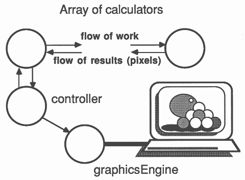
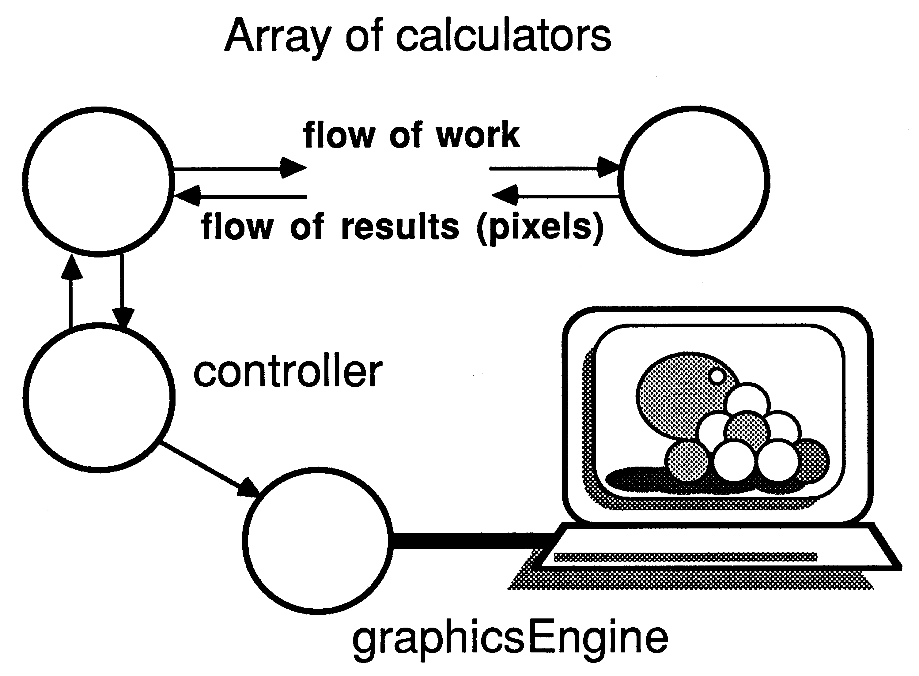
Here is a diagram of the ray tracer.
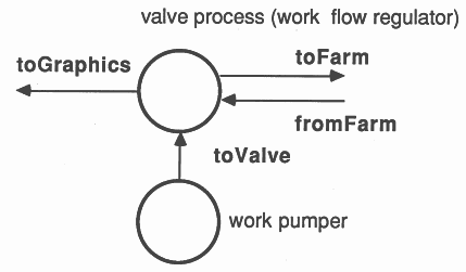
The key to the processor farm is a valve process, allowing work packets into the farm only when there is an idle processor. The structure of this valve is
PAR
-- pump work unconditionally SEQ i = 0 FOR workPackets inject ! packet -- regulate flow of work into farm SEQ idle := processors WHILE running PRI ALT fromFarm ? results idle := idle + 1 (idle > 0) & inject ? packet SEQ tofarm ! packet idle := idle - 1 |
where the crucial statement is the guarded ALT,
(idle > 0) & inject ? packet
|
only allowing work to pass from the pumper into the farm when there is an idle processor. The ALT is prioritised to accept results - this is explained in section 5.3.
The processor farm technique has been used to implement a very fast Mandelbrot Set generator [5][10] and a step-coverage simulator for VLSI circuits [9]. A large forecasting/statistical modelling package is in the process of being implemented as a processor farm. In all cases fully implemented, linearity of performance to number of processors has been high, from 80-99.5%. That is, ten processors perform between 8 and 9.95 times as well as one processor.
Ray tracing [8] is a computer graphics technique capable of generating extremely realistic images. It handles inter-object reflections, refraction and shadowing effects in a simple and elegant algorithm. However, ray tracing has one major drawback - it devours computing resource. In [8] very simple scenes were rendered on a powerful minicomputer, taking from 45 to 180 minutes per image.
The structure of the INMOS ray tracer was described in [4] and [5] - in this section the performance enhancement techniques described above will be illustrated with reference to the ray tracer.
Finally, results will be presented comparing the optimised implementation of the ray tracer with deliberately de-tuned versions.
As described in section 4 and in [4], the ray tracer consists of three major processes - controller, calculator and graphicsEngine.
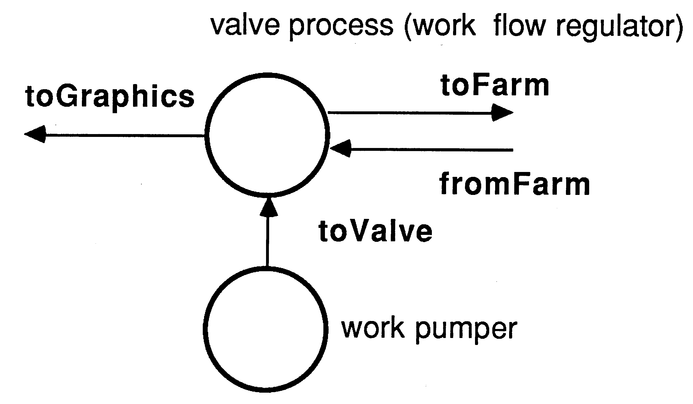
The controller is at the heart of the processor farm. The internal structure of the controller is illustrated below.
The valve process is regulating the flow of work into the farm of calculators, and passing results packets on to the graphics card. It is very important that the controller responds quickly to incoming results packets. Therefore the process accepting results packets is prioritised, and the ALT construct in the valve process is prioritised to accept results rather than pass on work. Each calculator has a buffered work packet, so it is more important that results be passed on to the graphics card rather than more work packets passed out to the farm.
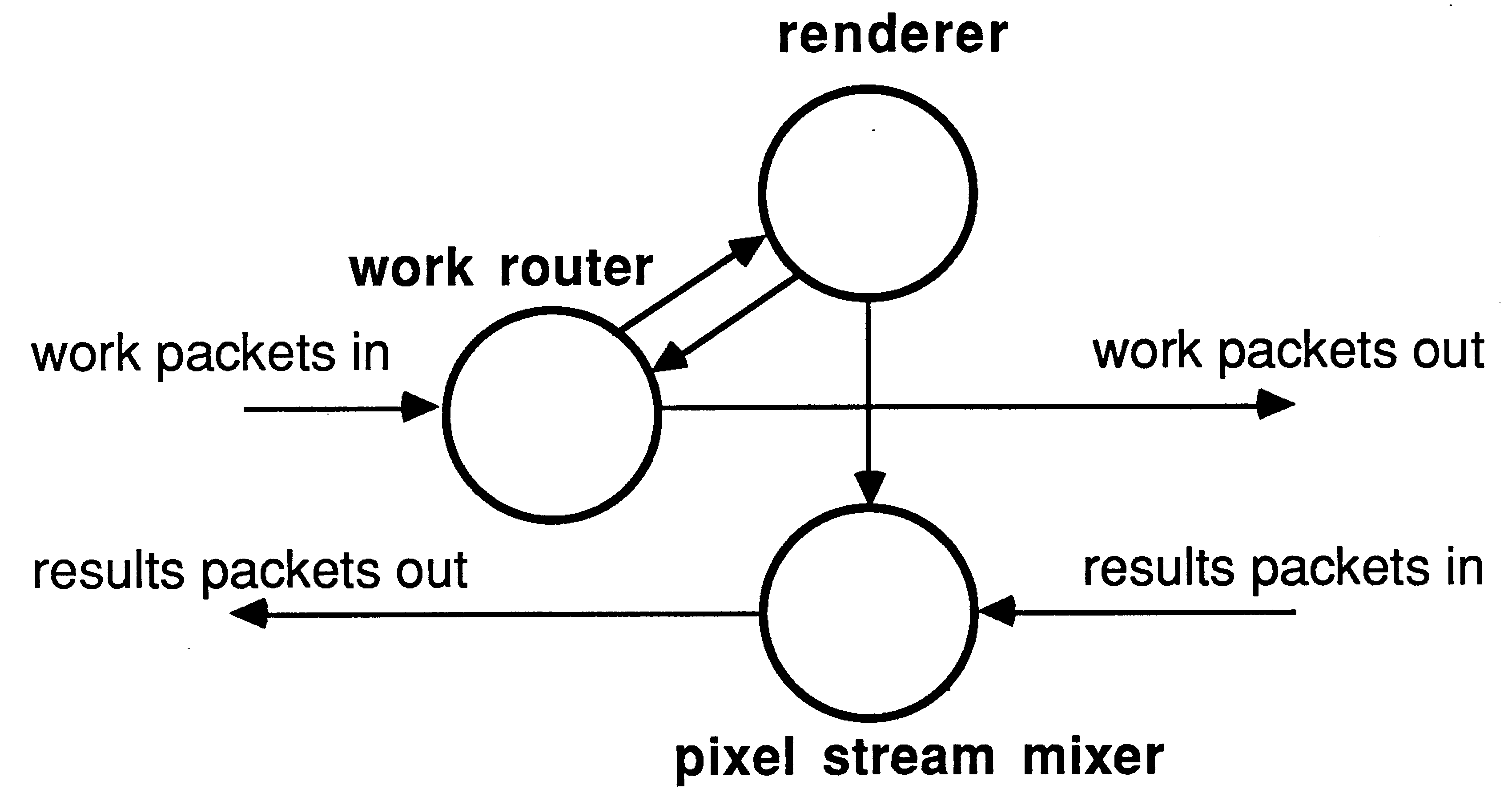
The calculator contains a work router, a pixel stream mixer and a renderer (section 3.1.2).
All the vectors used by mixPixels routeWork and calculate are declared at the outermost lexical level, and passed into the processes as parameters. Keeping the workspace of the work routing processes in internal memory is very important in a processor farro, as the latency of response to link inputs is reduced. When a process is scheduled, several words are written into the workspace of the descheduled process, and these write cycles will be slower if the workspace is off-chip, thus increasing process-swap time and degrading the performance of the farm as a whole.
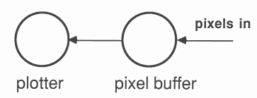
The graphics process accepts pixels from the controller and plots them on a B007 graphics board [7]. The internal structure of the graphics process is illustrated below.
The buffer process in graphicsEngine improves overall performance slightly, by overlaying the plotting of one patch with inputting the next. The buffer process is prioritised over the plotter.
To test the actual performance degradation due to non-adherence to these techniques, several deliberately de-tuned versions of the ray tracer were built, each omitting one or more of the enhancements described above. The results are presented below.
| Features | Timings | Relative degradation |
| None (fully optimised) | 143.28s | 0.00% |
| Inappropriate buffering (see 3.1.1) | 143.47s | 0.13% |
| No global vectors | 190.74s | 33.12% |
| No prioritised communications | 156.56s | 9.27% |
| All above | 199.87s | 39.50% |
| Prioritised computation | 1862.39s | 1299.80% |
Note the appalling performance (a factor of 13 degradation!) when computation is prioritised at the expense of communication. Throughrouting of data can never occur, and most of the processors are idle for most of the time, as they can neither off-load their results nor input new work packets, as the computing processes on their neighbours are not allowing the communications processes to be scheduled. This is obviously a gross mistake.
A more subtle mistake is the omission of prioritisation altogether. The figures quoted above are for 16 processors, resulting in a 9% degradation in performance. This figure gets worse as the ratio of communication to computation increases, and this ratio increases linearly with the number of processors in the array.
Several techniques have been presented for performance enhancement of occam programs running on transputers.
These techniques can be summarised as
| Enhancement technique | Section |
| Declare large vectors at the outermost lexical level | 2.1.3 |
| Use abbreviations to minimise static chaining | 2.1.3 |
| Use abbreviations to remove range checking | 2.1.6 |
| Use abbreviations to accelerate byte manipulation | 2.1.7 |
| Use abbreviations to open out loops | 2.1.8 |
| Place critical vectors on-chip | 2.1.9 |
| Clear large vectors with block move | 2.2 |
| Use TIMES | 2.3 |
| Decouple communication and computation | 3.1.1 |
| Use buffer processes on links where necessary | 3.1.1 |
| Prioritise processes which use links | 3.1.2 |
| Keep messages as long as possible | 3.1.3 |
| Use dynamic load balancing if appropriate | 4 |
Some techniques (dynamic load balancing, link buffering, buffer process prioritisation) are applicable only to arrays of transputers, others (optimum use of on-chip memory) should be applied at all times.
It has been shown that severe performance degradation can occur if an occam program is written without appropriate application of these techniques. Therefore these techniques should be considered for all occam applications.
Occam does not allow recursion, so recursive algorithms must be restated in a non-recursive manner. A good example is the anti-aliasing algorithm from the ray tracer.
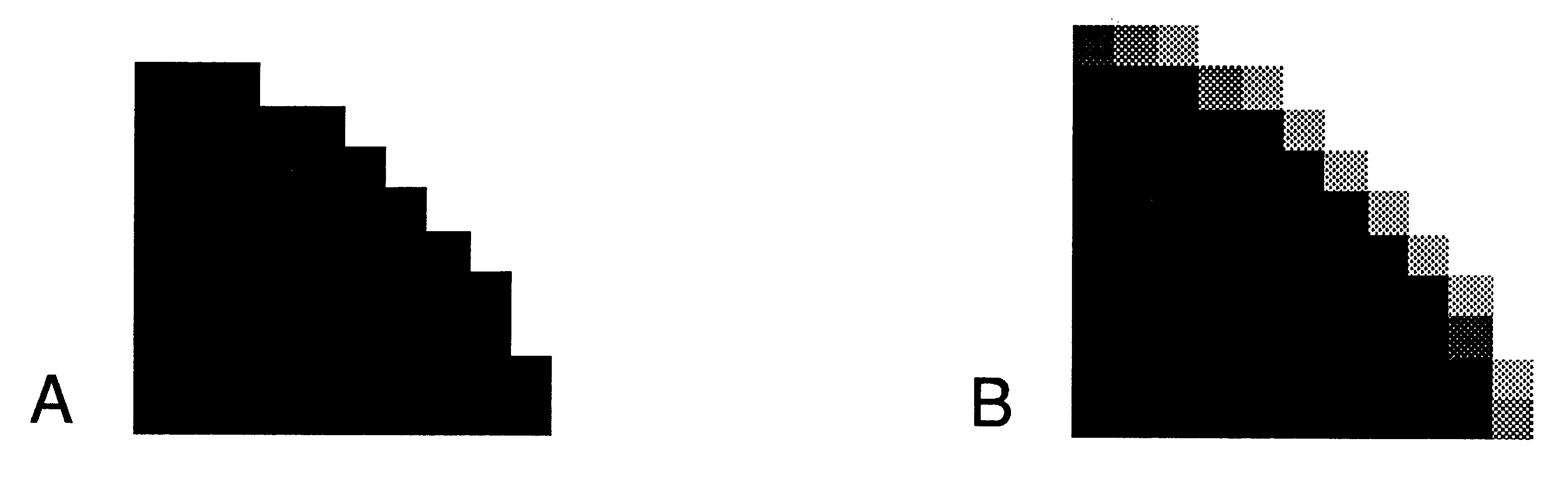
In computer graphics, anti-aliasing is a term used to describe algorithms which reduce perceptually disturbing artefacts in images. These artefacts are aliases, and are due to the point-sampling nature of computer graphics algorithms (see [8]). In order to reduce these aliases (and hence generate more realistic images) it is necessary to perform area-sampling, so that the colour assigned to each pixel on the display is an integration over the entire pixel area, rather than a single point sample.
The simplest approach to anti-aliasing is therefore to supersample each pixel (e.g trace 16 rays rather than 1) and return the average colour - this implies a factor of 16 increase in the work load, over-an already compute-intensive algorithm. Therefore an adaptive supersample is performed.
The purpose of adaptive supersampling is to generate an anti-aliased image without the expense of supersampling all pixels in the image. The algorithm supersamples those pixels where detectable colour changes have occurred, splitting these pixels into four sub-pixels and recurring. This results (in most cases) in an acceptable image at an average 30-50% increase in computation time, over a simple ray ’trace.
Expressed recursively in PASCAL, the algorithm is
FUNCTION averageColour ( x0, y0, size, level : INTEGER) : INTEGER;
FORWARD; FUNCTION averageColour ( x0, y0, size, level : INTEGER) : INTEGER }; VAR A, B, C, D, half : INTEGER; BEGIN A := rayTrace ( x0, y0); B := rayTrace ( x0+size, y0); C := rayTrace ( x0, y0+size); D := rayTrace ( x0+size, y0+size); IF (level < maxLevel) AND (colourDifference ( A, B, C, D) > maxDiff) THEN BEGIN half := size / 2 averageColour := ( averageColour ( x0, y0, half, level+1) + averageColour ( x0+half, y0, half, level+1) + averageColour ( x0, y0+half, half, level+1) + averageColour ( x0+half, y0+half, half, level+1)) / 4; END ELSE averageColour := (A + B + C + D) / 4; END; |
The recursion bottoms out either when a maximum recursion level has been reached, or when the colour difference across the corners of the pixel is deemed acceptable. The INMOS implementation has the maximum recursion level set to 2, so up to 16 rays will be traced per pixel for anti-aliasing.
In occam, the implementation is more verbose, but is simple to understand. The program explicitly manipulates 2 stacks - actions (i.e what the program should do next) and parameters (i.e the data on which the program shall act) are stored on one stack, and returned results (in this case colour values) are kept on the other.
An action value is popped off the stack and the appropriate action performed. If a TRACE action is to be performed then four points (representing the corners of the pixel) are raytraced, and their colours compared - if the colour spread is acceptable then the average colour is pushed onto the colour stack, otherwise a MIX action and four further TRACE actions are pushed onto the action stack.
If a MIX action is to be performed, four colour values are popped off the colour stack, and their average pushed back.
The algorithm terminates on a HALT action, at which time the pixel’s colour is held on top of the colour stack.
PROC averageColour ( INT averageColour,
VAL INT x0, y0, size0 ) ... declare actions - HALT MIX a b c d and TRACE x0 y0 size level ... declare variables, declare stacks, sp ... procs to manipulate action / parameter stack ... procs to manipulate colour stack SEQ ... init stack pointers push1Action ( HALT ) -- pre-load stack with HALT action push4Action ( x0,y0,size0,1) -- and parameters for this pixel action := TRACE WHILE action <> HALT IF action = TRACE INT a, b, c, d, diff : SEQ pop4Action ( x, y, size, level ) rayTrace ( a, x, y ) rayTrace ( b, x+size, y ) rayTrace ( c, x, y+size ) rayTrace ( d, x+size, y+size ) colourDifference ( diff, a, b, c, d ) IF (level < maxLevel) AND (diff > maxDiff) SEQ size := size / 2 level := level+1 push1Action ( MIX ) push5Action ( TRACE, x, y, size, level ) push5Action ( TRACE, x+size, y, size, level ) push5Action ( TRACE, x, y+size, size, level ) push4Action ( x+size, y+size, size, level ) TRUE SEQ push1Colour (((a + b) + (c + d)) / 4) poplAction ( action) action = MIX INT a, b, c, d : SEQ pop4Colour ( a, b, c, d ) push1Colour (((a + b) + (c + d)) / 4) pop1Action ( action) pop1Colour ( averageColour) : |
Note that as presented the algorithm is extremely inefficient, re-ray tracing points several times over. The algorithm as implemented caches previous results (in a large vector declared at the outermost lexical level and abbreviated into a local variable).
[1] Transputer reference manual, INMOS Limited, Bristol
[2] ”Occam 2 Language Definition” INMOS Technical Note David May, INMOS Limited, Bristol
[3] ”The Transputer Instruction Set - A Compiler Writers’ Guide”, INMOS Limited, Bristol
[4] ”Exploiting concurrency; a ray tracing example” INMOS Technical Note, INMOS Limited, Bristol
[5] ”Communicating Process Computers” INMOS Technical Note, INMOS Limited, Bristol
[6] ”IMS B004 IBM PC add-in board” INMOS Technical Note, INMOS Limited, Bristol
[7] ”IMS B007 A transputer based graphics board” INMOS Technical Note, INMOS Limited, Bristol
[8] ”An Improved Illumination Model For Shaded Display” Turner Whitted, Communications Of The ACM, pp. 343-349, June 1980, 23 (6).
[9] ”Evaporated film profiles over steps in substrates” I.A Blech, Thin Solid Films, 6 (1970) pp 113-118
[10] ”Turbocharging Mandelbrot” Dick Pountain, BYTE magazine, September 1986
[11] ”Signal Processing With Transputers” J.G. Harp, J.B.G. Roberts and J.S. Ward Computer Physics Communications January 1985