|
|
| Communicating Process
Computers
_____________________________________________________________________ |
| David May and Roger Shepherd February 1987 |
This paper is concerned with the construction of computers based on communicating process architecture. We wish to establish that this architecture is practical and that it is feasible to build a general purpose computer based on this architecture. We shall start by looking briefly at the technological background and the questions that this raises, then look at a number of real applications, and finally we will discuss the possible structure of a general purpose parallel computer.
At the present level of VLSI technology we can implement in the same area of silicon the following components of a computer:
Consequently, using the same silicon area, we can construct a single 10 MIPS processor with 4 MBytes of memory (a conventional sequential computer) or a 10000 MIPS computer with 2 MBytes of memory. Both machines would require about 1000 VLSI devices, and so are quite small computers.
The problems are now to decide on the correct ratio of memory to processors and how to construct a system with many processing elements with small amounts of memory dispersed through the system, in such a way that it can be applied to practical problems. Obviously, a collection of 1000 or more processing elements must be arranged in a regular structure, and a number of different structures have been proposed. Examples are:
These structures vary in three important respects:
We will return to these matters when we consider the implementation of applications on general purpose communicating process computers. But first we will look at some applications.
We now look at a number of applications where the concurrent implementation seems to dictate a specific processor structure. All these applications have been developed and actually run on multi-transputer systems. The examples are divided into three groups. The first group contains applications where the parallelism has been obtained by decomposing the algorithm into a number of smaller, simpler components which can be executed in parallel. The second group contains applications where the parallelism has been obtained by distributing the data to be processed between a number of processors in such a way that the geometrical structure of the data is preserved. The final group contains applications where a number of processors are used to process data farmed out by a controlling processor. Of course, these groups are not mutually exclusive, and our solid modelling application shows aspects of both algorithmic and geometric decomposition.
In the following two examples the algorithm used follows from a dataflow analysis of the application and the parallelism arises directly from that algorithm.
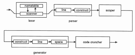
The first example is the occam-in-occam compiler. One of the reasons for the choice of this example is to illustrate that concurrency can arise where it might not be expected. In order to write this compiler concurrently (deliberate ambiguity!) a dataflow approach was taken; the parallel decomposition of the algorithm then follows straightforwardly. The diagram below shows the structure of the compiler.
|
|
From the outside, the compiler appears to be a single pass compiler. Internally, it is more like a multiple pass compiler; each process performs a simple transformation on the data which flows through it. For example, the lexer process inputs a sequence of characters and outputs a sequence of tokenised lexemes. It is able to do this continuously; as soon as it has recognised a sequence of characters as a lexeme it is able to output the appropriate token.
The effect of decomposing the compiler in this way was that each component process was relatively easy to write, specify and test; this meant that the component processes could be written concurrently! Also, as the machine dependencies were restricted to the final stages of the compiler, it was possible to develop the compiler for different targets concurrently.
The occam program for the compiler is outlined below:
-- occam compiler
CHAN lexed.program: CHAN parsed.program: CHAN scoped.program: CHAN coded.program: PAR -- lexer CHAN name.text: CHAN name.code: PAR ... scanner ... nametable -- parser CHAN parsed.lines: PAR ... line parser ... construct parser ... scoper -- generator CHAN generated.constructs: CHAN generated.program: PAR ... construct generator ... line generator ... space allocator ... code cruncher |
The program, as shown, could be executed on a pipeline of processors. However, it is unlikely that it will offer an increase in speed which is proportional the number of processors used.
There are two important reasons for this. The first is that the throughput of a pipeline is limited by the throughput of the slowest element of the pipeline. This means that in order to have the potential for maximum multi-processor speed-up a pipeline must be ’balanced’; that is each component of the pipeline must process data at the same rate. The compiler pipeline is not balanced; measurements show that the code cruncher accounts for about 40% of the processing resource used. The second reason is that the pipeline does not contain sufficient buffering to allow each individual stage to operate as fast as possible. For example, the line parser operates on a line of lexemes at a time, whereas the lexer operates on only a lexeme at a time. This means that without a buffer inserted between the lexer and the line parser, the lexer will halt whilst the line parser transforms a line.
Another example of an application for which the algorithm decomposes easily is solid modelling. This involves the generation of shaded images of polygonal objects in real time. This has application in the areas of Computer Aided Design and Computer Animation.
For each object the following steps are performed. First the object is translated into the ’world space’ (the world space defines the spatial relationships between the objects to be modelled). The object is then transformed into the ’image space’, this involves rotating and projecting the object so that it will appear in proper perspective as seen by an observer at the chosen ’viewpoint’. The image of each object must be ’clipped’ to the screen and then ’drawn’ into a Z-buffer which is used to resolve depth. The algorithm can be extended to provide animation by allowing the objects, the world, and the viewpoint to change for each frame.
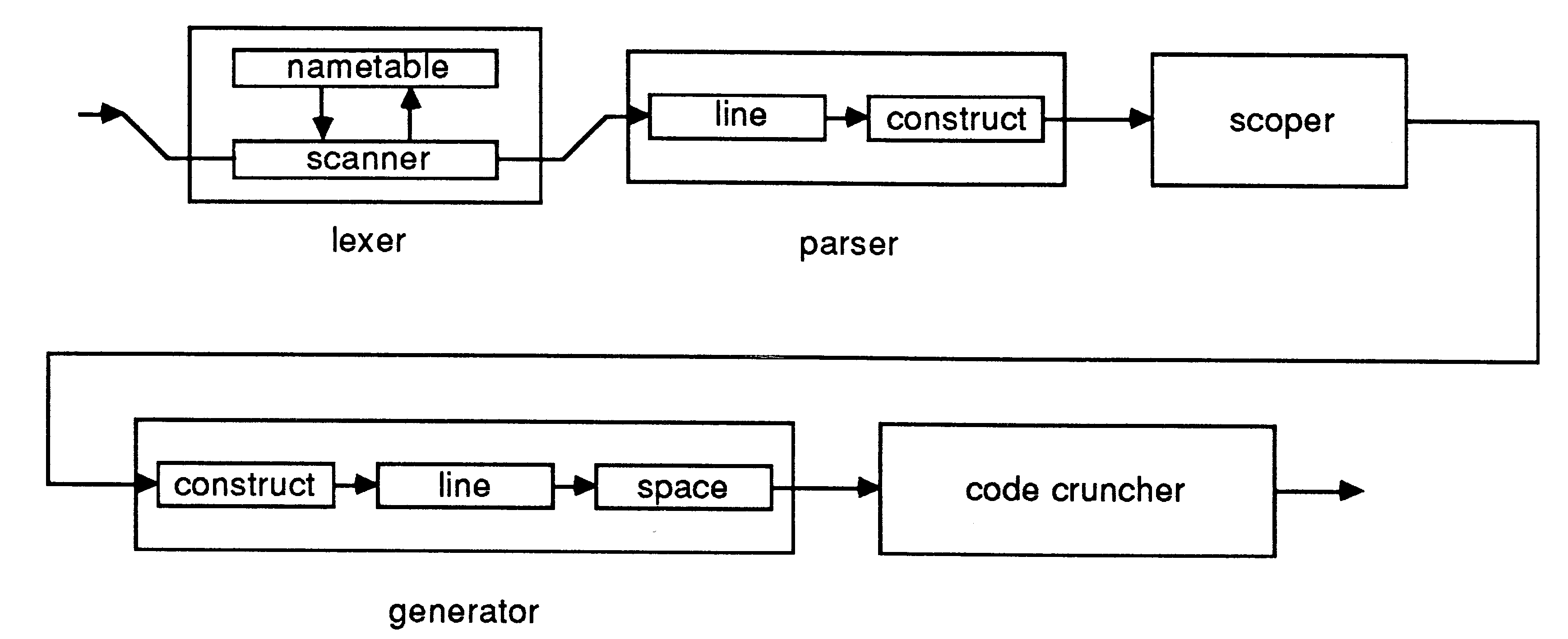
At the top level we choose to implement the algorithm as shown in the diagram below.
|
|
Here each object is passed to a transformer which passes the transformed object to the drawing process. We use several transformers to increase the rate at which we can draw objects. As a transformer becomes free, the object store can send it another object to transform. In this way we obtain a linear multiprocessor speed up; n-transformers can process data at n-times the rate that one transformer can. This speed-up is predicated on the object store being able to supply objects at a great enough rate and on the drawing process being able to draw objects fast enough.
We can now turn to the implementation of the transformation process. The sequential implementation of this process could be written as:
WHILE active
SEQ from.object.store ? object world(object) viewpoint(object) clip(object) to.drawing.process ! object |
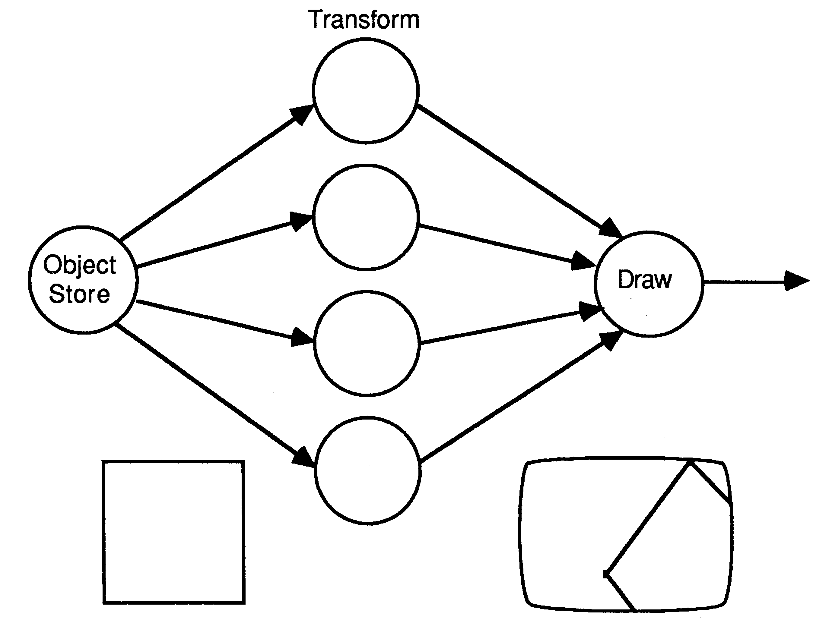
This process can be distributed over a pipeline:
|
|
The program becoming:
CHAN world.to.viewpoint :
CHAN viewpoint.to.clip : PAR ... world ... viewpoint ... clip |
The parallel processes would all have the same general form; for example, the viewpoint process would be:
WHILE active
SEQ world.to.viewpoint ? object viewpoint(object) viewpoint.to.clip ! object |
In practice these processes would be probably be more complex than the program above suggests, we would want to introduce buffering so that the whole of the transformation pipeline could be kept busy.
In the example below use is made of the geometric structure of the data to distribute the application onto a number of processors.
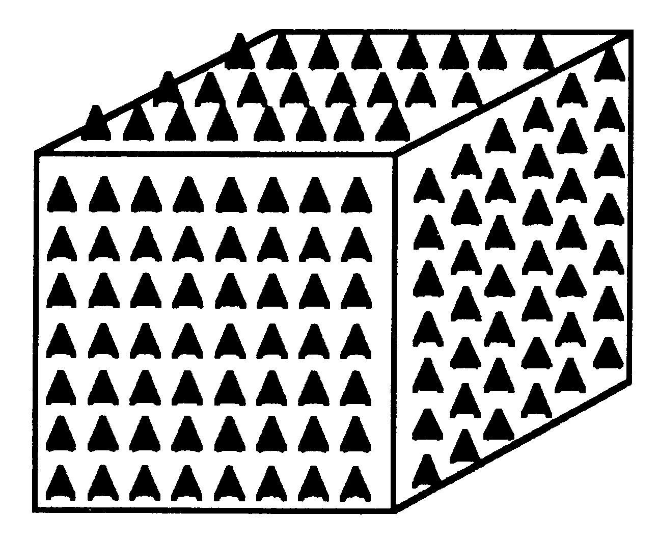
Statistical mechanics is the study of mechanical systems where the behaviour of the components is described statistically and cannot be resolved analytically. A familiar example of a statistical mechanical system is provided by the magnetic properties of iron. For this purpose iron can be modelled as a cubic lattice of small magnets.
|
|
The orientation of these magnets is known as a spin because the magnetism is related to the spins of the electrons in the iron. This model is thus called a 3-dimensional spin system.
We can simulate the behaviour of iron on heating by examining what happens to the lattices over successive time steps as it is heated. During each time step there are two important influences on each small magnet. Firstly, there are thermal vibrations which will tend to move the magnet away from its current orientation. The thermal effects are described statistically, with the distribution being dependant on the temperature of the iron. The second influence will be the magnetic forces applied by the neighbours of the magnet under consideration. If we start with a magnetised lattice and raise the temperature the thermal effects will eventually overcome the magnetic forces and the lattice will become disordered and thus demagnetised.
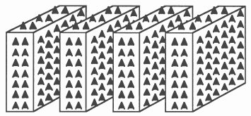
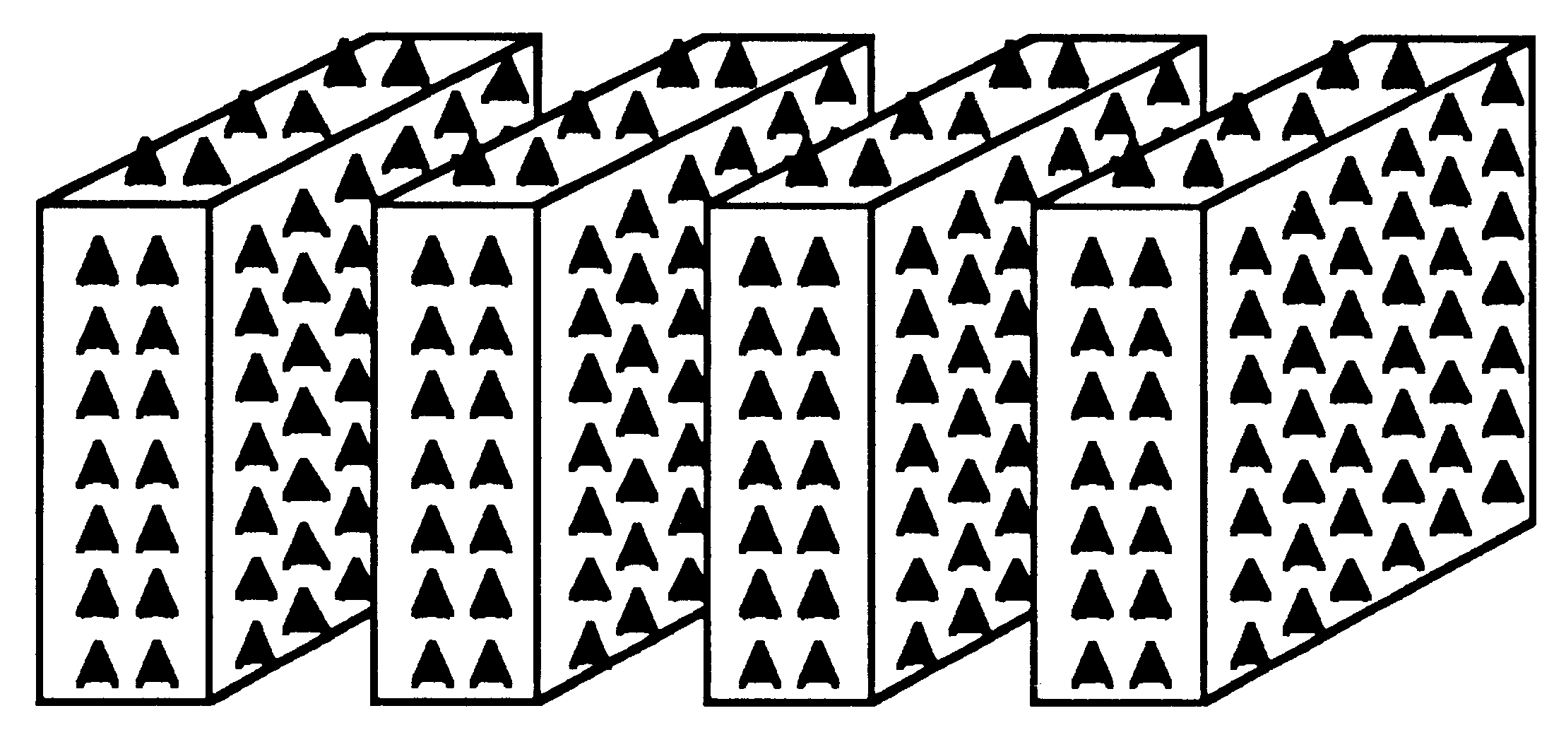
It is easy to see that a statistical mechanical system can be decomposed in terms of its natural geometrical structure. For example, the cubic lattice of iron could be split between a number of transputers, each dealing with a small portion of the problem. Each transputer can then update that part of the lattice for which it contains the data. Communication will be needed with neighbouring transputers so as to exchange information about adjacent lattice sites which are placed on different transputers.
|
|
We will now look at a practical example of a statistical mechanical simulation. This is a simulation of a generalised planar spin model (i.e. a 2-D spin system) with both ”Exchange” and ”Nematic” interactions [1] which has actually been implemented on a number of transputers. The system can be interpreted in terms of liquid crystal films; however, the major interest in the system is theoretical in that it exhibits an unusual phase structure.
The program operates on an L x L square lattice of spins with periodic boundary conditions. The spins are represented by angles which are discretised to lower the storage requirements and to allow a table look-up for fast cosine generation.
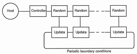
The original aim of the design was for the system to be implemented on an array of transputers without any external memory. This imposed a large constraint because the straightforward geometric decomposition of the updating process gave rise to a collection of processes each of which was too large to reside in the memory of a single transputer. The solution was to split the updating work into two parallel processes, ’random’ and ’updata’ each of which could fit on a transputer.
|
|
The random process generates uniformly distributed and exponentially distributed random numbers and communicates with the controller process. The updata process performs the rest of the updating algorithm, stores data (512 spins) and computes correlations. Each random/updata pair of processes implements a vertical ‘strip’ of the lattice. Horizontal communication is required for the interaction of the spins on the vertical edges of the strips.
In practice the ’no-external memory’ requirement was relaxed. The program was run at INMOS on 17 transputer evaluation boards (each board having an 80 ns cycle time transputer with external memory). The extra memory permitted the random and updata processes to be implemented on a single transputer, the lattice to be decomposed into 16 4 x 64 strips, and the discretisation of the spins to be increased to 128 states as the size of the cosine table could be enlarged.
The efficiency of the simulation was:
time of program on 1 processor
-------------------------------------- = approx 80% 17 x time for program on 17 processors |
The simulation, which took about 60 hours to run, would have taken about 3 months on a VAX 11/780.
The Mandelbrot set, M, is the set of complex numbers:
| M = {c : |Mn(c)| < ∞ ∀n ∈ N} |
where:
| M0(c) | = 0 | ||
| Mn+1(c) | = Mn(c)2 + c |
It can be shown that if ∃n : |Mn(c)| > 2 then c not ∈ M.
The edges of the Mandelbrot set are intricate, and, because complex numbers can be represented on a two-dimensional plane, the set can be plotted on a graphics screen with impressive results. In practice, the colour of each pixel on the screen represents whether or not the corresponding point of the complex plane is in the Mandelbrot set. If a point is not in the Mandelbrot set then the colour plotted at that point represents the number of applications of the recurrence required to determine that it is not in the set. A point will be considered to be in the set if the recurrence has been applied more than a fixed number of times (for example 1000) without the modulus becoming greater than 2.
For a given point (x,y) the following process applies the recurrence until a colour can be chosen.
iterations := 0
z := COMPLEX(0.0, 0.0) WHILE (iteration < 1000) AND ((MOD z) < 2) SEQ z := (z*z) + COMPLEX(x, y) iteration := iteration + 1 |
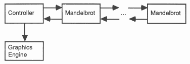
To plot a picture of the Mandelbrot set requires that we perform the above process for every pixel on the screen. However, as the computation for each pixel is independent we may perform it for many pixels in parallel. The implementation we have chosen is shown in the diagram below:
|
|
The basic idea used in this implementation is that the controller process hands out a point to each Mandelbrot process. When a Mandelbrot process has computed the colour to be displayed at that pixel it sends the information to the controller which passes the pixel to the graphics engine and hands the Mandelbrot process another pixel. This approach is very attractive because the amount of computation required varies from pixel to pixel and this implementation automatically balances the load.
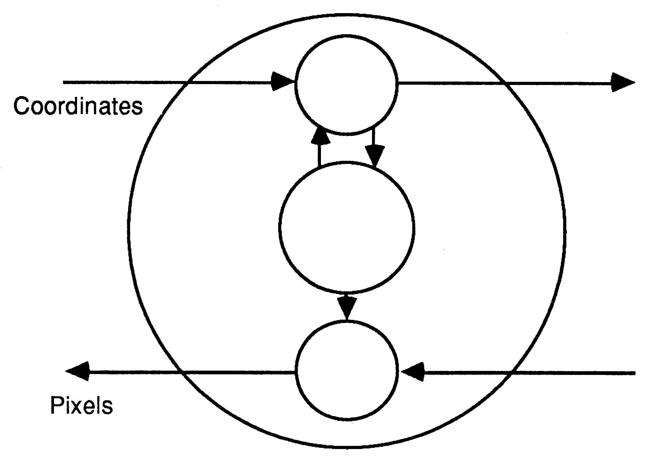
As can be seen from the previous diagram, Mandelbrot processes not only compute the colour for a pixel but they also provide a means for the controller to communicate with Mandelbrot processes to which it is not directly connected. The structure of the Mandelbrot process is as shown below:
|
|
This implementation turns out to be quite effective. If there are N processors available to execute Mandelbrot processes then an upper bound on the amount of communication required for each pixel will be 10 x N bytes. This is not a large amount considering that the computation for each pixel may require up to 2000 operations on floating point complex numbers.
It turns out that in order to keep the processors busy the Mandelbrot process has to buffer an extra item of work so that when it completes the computation for a pixel it can start on its next pixel at once rather than having to wait for the controller to send it the next item of work. In the diagram above the extra work is buffered in the router, and when the Mandelbrot computer process finishes its computation it sends a message to the router requesting more work.
The algorithm sketched above can be improved upon so as to decrease the number of interactions between the controller and the Mandelbrot processes by handing each Mandelbrot process more than a single pixel as its item of work. In practice we have chosen to use a quarter of a scan line as the unit of work. We have found that the communication cost with this approach is insignificant even with tens of processors connected in the manner shown.
Whilst the previous example of a computer graphics application may seem a little artificial and especially suited to parallel implementation this example is very real. A large amount of super-computer time is spent on this application by people such as film makers.
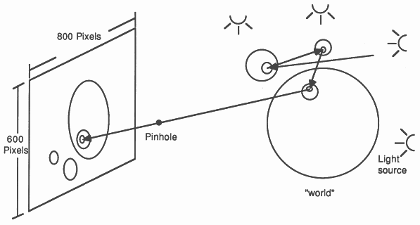
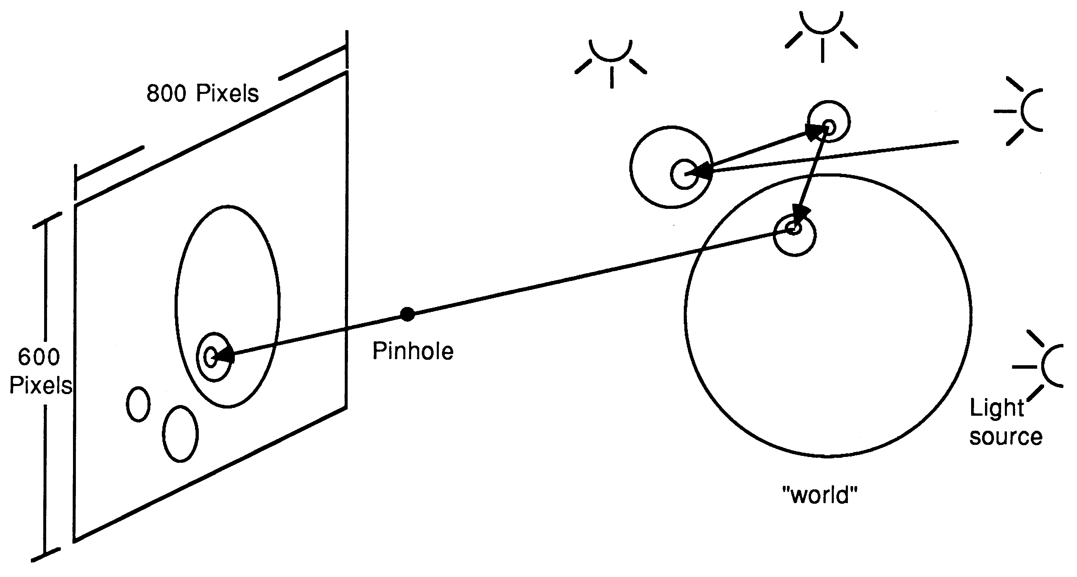
The application is ’ray tracing’. This is a means of producing very high quality, life-like computer graphics. It is capable of correctly representing reflective and refractive objects (mirrors and lenses) and light sources.
|
|
The way in which the technique works is to take a point on the screen and to produce the ray that would arrive at that point from a pinhole sitting between the screen and the objects to be drawn. The ray is then extended into the object space and intersected with each object in the space. The first object with which the ray intersects is determined. In the simplest case this object will be matt and the colour of the object is plotted at that point on the screen. If the object is reflective, the path that the ray would take after reflection is computed and the process repeated. The same general principal allows the pin-hole to be replaced by a lens, giving depth-of-field effects.
It may now be seen that the basic structure of the problem is essentially the same as plotting the Mandelbrot set. For each point on the screen a colour has to be generated. The computation for each point is independent and computationally intensive. Ray tracing, can, therefore, be implemented on exactly the processor structure as was used for drawing the Mandelbrot set.
It is quite interesting that the previous two examples are implementable on exactly the same configuration of processors. It is also interesting that these configurations actually seem to have nothing to do with the application in hand.
In fact further consideration of both these algorithms will show that almost any configuration of processors will do subject to it providing sufficient communication capability. Both these applications have two distinct parts; the first farms out work to a of number application specific processes, the second is the application specific process. We call this type of arrangement a processor farm.
From the last two examples we have seen that there are applications which are basically insensitive to the arrangement of processors on which they are run. Of course, there is the proviso that the arrangement of processors must provide sufficient communication capability. As we now have evidence that it might be reasonable to try and construct a general purpose structure of processors we can return the issues raised in the introduction.
Pipelines and simple (2 dimensional) arrays can be easily implemented or extended. Arrays (and hypercubes) become progressively more difficult to implement as the dimension increases, with much space taken by connections which need to cross over. However 1000 or so processing elements can be connected in this way.
One difficulty with the hypercube structure is that the number of links provided at each node must be at least the dimension of the hypercube. This means that a standard component (which has a fixed number of links) cannot be used to implement an arbitrarily extensible array. An alternative structure which avoids this problem is obtained by implementing each node of the hypercube with a ring of transputers – this structure is known as ’cube connected cycles’. The cost of non-local communication, which arises when two nodes need to communicate via intermediate nodes, varies widely. A one dimensional array is obviously the worst. It is clearly desirable that the worst case path between two points (the ’diameter’) of the network is small in relation to the number of nodes, and several structures have this property:
| structure | diameter | size |
| hypercube | ∼ n − 1 | 2n |
| cube-connected cycle | ∼ (n × 5)∕2 | n × 2n |
| folded tree | ∼ n | n × 2n−1 |
If such a structure is being used, for example to implement a processor farm, it may be necessary to implement a routing algorithm. It is quite easy to design. a general purpose algorithm for this purpose but for many applications an application specific router may be better.
An example of a routing process is shown below
... declarations
SEQ ... initialisation WHILE active SEQ ALT ALT l = 0 FOR 4 link.in[l] ? message SKIP internal.in ? message SKIP dest := route.table(message(0]] IF dest = internal internal.out ! message TRUE link.out[dest] ! message ... check for termination |
The above routing process inputs a message from a link or from the process co-resident on the transputer. The process examines the first word of the message to determine the destination, and looks up that destination in a route table which identifies whether it should be sent to the local process or re-transmitted down a link.
More complex versions of the routing process would enable the transputer’s links to operate concurrently. However, they would almost certainly impose a larger overhead on the processor’s computing power, and thus might be suitable for algorithms where the required communication bandwidth is relatively high.
Normally the routing process in a transputer would be prioritised over other processes. This ensures that when a message arrives at the routing process it is inspected (and forwarded if necessary) immediately it is received. If a high priority process were not used the message would not be examined until the routing process was executed on the round-robin.
Although a routing process has an impact on the computing power available at each node, once a data transfer has been initiatated the transputer’s autonomous links will transfer the data without the further intervention of the processor. This means that the processor resource used by a routing process is dependent on the number of communications rather than the quantity of data transmitted in each communication. This in turn suggests that the correct strategy is to maximise the length of message passed at one time.
On the other hand, where the length of time it takes for a message to reach its destination is critical, there are advantages in breaking data into small messages. This enables several processors to transfer the data concurrently. This is also true where it is necessary to broadcast data throughout an array. These matters have been investigated elsewhere in the literature [2].
For a given problem, it is usually possible to adjust the processing time per communication by use of a combination of parallel and sequential algorithms. At one end of the spectrum is the ’data flow’ program with many simple processes each of which inputs a message, performs a single operation and outputs it; at the other end is a sequential program which inputs a message, performs many operations, and outputs the result. One of the advantages of a communicating process language is that it combines both sequential and parallel programming techniques, and one of the uses of program transformations is to perform this kind of optimisation.
It is possible to write programs in a manner whereby the granularity of the computation is easy to adjust. For example, in the Mandelbrot set drawing program it is easy to alter the granularity from a single pixel (large potential for parallelism) to a whole screen (small amount of communication). This is useful because the communication to computation ratio can vary as hardware changes. For example, the introduction of the floating point transputer will drastically reduce the computation load of a transputer which is drawing the Mandelbrot set. As result of this, the program should be altered to increase the number of pixels computed at a time.
Experience suggests that many numerical problems can be organised so that communication times are dominated by computing time. For example, a process which inputs two n × n arrays, and outputs the product involves 3 × n2 communications but the multiplication involves n3 operations.
Given a general purpose structure. such as a 2 dimensional array, it is obviously possible to use a number of different techniques to implement an application. For example, a number of applications could suit either a pipeline or processor farm implementation.
The question then arises as to which implementation is preferable. There are a number of considerations here:
We would like to give one final example of a processor farm implementation. The application we have chosen is producing the sum of all prime numbers less than a specified number. We calculate this by producing all prime numbers less than the specified number and summing them. The prime numbers are produced by successively testing the primality of odd integers. We test the primality of an integer n by dividing by primes up to sqrt(n) .
This problem is of interest because it contains the sequential dependency that an number n cannot be tested for primality until we have tested all numbers up to sqrt(n) . We have chosen a very simple solution to this problem for the sake of exposition.
We distribute the problem by having a number of processors running primality testers and a single controller processor. Each primality tester maintains a list of prime numbers, supplied to it by the controller process. It uses this list to determine the primality of candidates passed to it by the controller. The controller ensures that when a primality tester tests a candidate n the tester contains all primes up to sqrt(n) .
The program for the primality tester is:
... initialisation
WHILE active SEQ from.controller ? object.type; object.value IF object.type = candidate VAR candidate.is.prime : SEQ IF IF i = 0 FOR primes.stored (object.value \ primes[i]) = 0 candidate.is.prime := FALSE TRUE candidate.is.prime := TRUE to.controller ! object.value; candidate.is.prime object.type = prime ... add to list of primes object.type = halt active := FALSE |
The program for the controller is:
... initialisation
problem ? upper.bound; root.upper.bound ... generate primes until prime > root.upper.bound WHILE next.candidate < upper.bound VAR nactive : SEQ ... hand out next batch of primes ... start primality testers nactive := ntesters WHILE nactive > 0 ALT i = [0 FOR number.testers] from.prime.test[i] ? resolved.candidate; is.a.prime SEQ ... add into prime sum if is.a.prime IF more.candidates ... send next candidate TRUE nactive := nactive - 1 ... terminate primality testers result ! prime.sum |
The inner WHILE loop hands out a new candidate to a tester in response to the tester returning the result of its previous test. The loop terminates when there are no more candidates which can be tested using only the primes currently stored by the testers.
The outer WHILE loop will then cause another prime to be supplied to all the testers and the testers to be restarted. This continues until all candidates less than the upper bound have been tested.
Although this solution requires a certain number of primes to be generated sequentially the program could be altered so that just sufficient primes were generated to ensure that the testers could start operating; that is, in order to sum primes up to n, primes up to sqrt(sqrt(n)) would be generated. At this stage the testers can start working and a further concurrent process could start generating the primes which become needed by the testers as testing continue.
It is also possible to make the controller maintain an ordered list of primes produced by the testers. The early primes produced can than be used in the testing of larger primes.
[1] Simulation of statistical mechanical systems on transputer arrays, C R Askew, D B Carpenter, J T Chaiker, A J G Hey, D A Nicole and D S Pritchard, Physics Department, University of Southampton, To be published
[2] Signal processing with transputer arrays, J G Harp, J B G Roberts and J S Ward, Royal Signals and Radar Establishment, Malvern, Worcestershire, Computer Physics Communications, 1985.