Contents

1 Introduction

The occam programming language [1] was developed by INMOS to express concurrent algorithms and their implementation on a network of transputers [2]. Data allocation in occam is static [3] so the exact data space requirement of a program is known after compilation, allowing the run time overhead of the parallel construct to be very small [4]. Recursion needs dynamic storage allocation so it is not directly implemented in occam. Also, occam does not directly support data structures such as trees, stacks and lists.

This technical note is designed to introduce some suggestions to occam programmers handling recursion and data structures. It will describe some common data structures and gives guides for implementing them in occam. It will discuss recursion and methods of transforming recursive algorithms to iterative ones. It will explore two methods of implementing recursion in occam and will give two simple examples to illustrate these methods.

Note that all occam examples compile on the occam 2 product compiler.

2 Data structures

Data structures are used to allow easy representation of the storage, retrieval and manipulation of information. The following sections give a brief introduction to the occam programming language then describe how some of the familiar structures may be implemented in occam. More information on data structures can be found in reference [11].

2.1 The occam programming language

The occam language enables a system to be described as a collection of concurrent processes which communicate with one another, and with the outside world, via communication channels. Occam programs are built from three primitive processes:

Each occam channel provides a one way communication path between two concurrent processes. Communication is synchronised and unbuffered. The primitive processes can be combined to form constructs which are themselves processes and can be used as components of another construct. Conventional sequential programs can be expressed by combining processes with the sequential constructs SEQ, IF, CASE and WHILE.

Concurrent programs are expressed using the parallel construct PAR, the alternative construct ALT and channel communication. PAR is used to run any number of processes in parallel and these can communicate with one another via communication channels. The alternative construct allows a process to wait for input from any number of input channels. Input is taken from the first of these channels to become ready and the associated process is executed.

2.2 Records

2.2.1 A common example

Records are collections of one or more data items, possibly of different types, grouped together for ease of handling. The traditional example of a record is that of an employee who is described by a set of attributes such as name, date of birth, salary etc. The attributes of a record are called the fields or members of the record. Occam allows clarity and easy manipulation of records and fields of records by using abbreviations and RETYPES, see reference [6].

2.2.2 Using arrays of INTS and RETYPES

Records may be implemented in occam by declaring an array to be the area of store for the record. By using abbreviation and the RETYPE instruction we can access the fields of the record. An implementation of occam will represent variables using a number of bytes in memory. The RETYPE instruction allows us to interpret this representation as a variable of a different type. This allows us to use a string of bytes as an integer, a real or a boolean value. RETYPES simply change the way in which a data item is viewed by the compiler.

RETYPES to REALs or to INTs must be word aligned, indeed, it is good practice to word align all RETYPES. This means that the area of store should be declared as an array of INTs, not BYTES, to ensure that the base of the array is correctly aligned, that the records should be padded out to ensure that the fields are correctly aligned and that each record should be a whole number of words. The product compiler checks that a retyped variable is correctly word aligned. Using RETYPES allows us more explicit control over memory allocation than in many languages (e.g Pascal), where automatic word alignment may mean bytes are wasted without the programmer realising.

For example, we could declare an array of 150 employee records, each record using 8 words of memory, and pass the first of those records to procedure UseRecord as follows:

The procedure UseRecord could access the fields of the record using the RETYPES and abbreviations below. Occam implements formal parameters as abbreviations for actual parameters [1]. Thus the parameter to the procedure abbreviates the particular record in current use, say Employee[0]. Such an abbreviation helps to make the action of the procedure clear. Abbreviations should also be used for the number of bytes each field requires and for the location in the array where each field starts; all, excepting NameSize and NameBase, have been omitted below for clarity.

The fields may then be used in the same way as variables, as illustrated in the initialisations below. The usage checker ensures no assignment or input is made to record directly because record was used to define the abbreviations and RETYPES.

In the example above the RETYPES to REALs and INTs have been word aligned. The first five words are used for the employees name, the first two bytes of the sixth word are the INT year and the last word is the REAL salary.

The costs incurred by a RETYPE are the initial overhead of setting up an abbreviation and, for those that might not be correctly aligned, the cost of an alignment check. Also, access to a retyped (or abbreviated) variable may be more expensive than access to a local scalar variable.

2.2.3 Protocols

Named protocols provide an easy way to pass records between concurrent processes. Referring to the example above, the whole record or the date of birth fields only may be passed using the following protocols.

2.2.4 Arrays for each field

Another method of implementing a collection of records is to use a different array for each field of the record. Thus the example given above would be implemented as follows:

Or, as a mixture of the two methods:

Using the RETYPES and abbreviations described below to access the different parts of the date of birth. This example uses the first record.

This will remove retype alignment problems but it will make protocols for communicating entire records a little more complex.

2.2.5 Avoiding alignment

Another way to overcome the problems of alignment is to use copying to achieve re-alignment of data. This involves providing a number of construction, destruction, enquiry and updating routines. This has the effect of ’hiding’ details of the record manipulation as much as possible. In some applications, where only a few fields are being examined, this method may be more efficient than locally abbreviating the fields wanted. Indeed, if the main data structure is stored in off-chip memory and the local variables being copied to are in on-chip memory, then access to the fields would be considerably faster.

The following routines require no alignment of data within the record, avoiding many possible pitfalls and minimising memory usage. A few examples are given (With thanks to Roger Shepherd), the construction of the rest should be obvious. The procedure Name.of.Person has not been implemented as a function because the rules of occam 2 only allow functions to return results of primitive data types, not array types. If your compiler release does not support functions then BirthYear.of.Person and other enquiry routines may be implemented as procedures in a similar manner to Name.of.Person.

2.3 Stacks

2.3.1 The stack data structure with associated operations

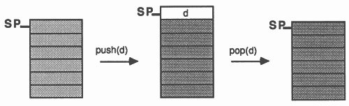
A stack can be visualised as a pile of objects. The top of the stack is the only place accessible, that is, objects are always taken from or put onto the top of the stack. A stack has three procedures and two boolean functions associated with it:

InitStack():

sets the stack empty by pointing the stack pointer sp, a free variable, to NIL.

pop(d):

assigns the value of the top element to d and removes it from the stack.

push(d):

places the value d onto the top of the stack.

StackEmpty():

returns TRUE if the stack is empty, FALSE otherwise.

StackFull():

returns TRUE if the stack is full, FALSE otherwise.

Figure 1 demonstrates these procedures.

2.3.2 Occam implementation

A stack may be implemented in occam by using an array to store the data items. The stack pointer is implemented by using an integer index to the array. For example, a stack to store a maximum of 100 integers, 1 integer at a time, could use the following code:

A particular program may use many different stacks, for instance one to hold parameters and another to hold results. The same subroutines may be used for the operations on different stacks by passing the stack pointer as a parameter to the subroutines. A stack can store more than one item, of any type, each time data is pushed on, indeed a stack can store records as described above. Similarly, more than one item can be popped off a stack at one time and two or more popping procedures could be used, say, one to pop two items off and another to pop three. Stacks may be made to grow from the top down instead of from the bottom up.

2.4 Queues

2.4.1 The queue data structure with associated operations

A queue is a list that may have items taken from the head of the queue or items added to the tail of the queue. Thus, the first item to be placed on the queue is the first to be taken off. It has three procedures and two boolean functions associated with it:

init.q():

empties the queue.

on.q(d):

puts the data item d at the tail of the queue.

off.q(d):

takes a data item off the head of the queue.

q.is.full():

returns TRUE if the queue is full, FALSE otherwise.

q.is.empty():

returns TRUE if the queue is empty, FALSE otherwise.

2.4.2 Occam Implementation

A queue may be implemented in occam by using an array to store the data. The two pointers to the head and tail of the queue are implemented by using integer indexes to the array. The array is treated as a circular store, that is, if we use an array of size q.size and we wish to store an item in queue[q.size] we would store it in queue[0]. Thus, when the tail is equal to the head, the queue is either empty or full. To distinguish between these two cases we will always leave a blank entry in the array. This means that when the head and tail are equal the queue is empty and when the head is one behind the tail the queue is full.

For example, a queue to store a maximum of 99 integers could use the following code:

Queues may, of course, be implemented to store and retrieve more than one data item at a time.

2.5 Linked lists

2.5.1 Linear lists

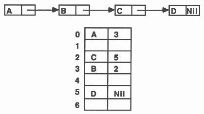
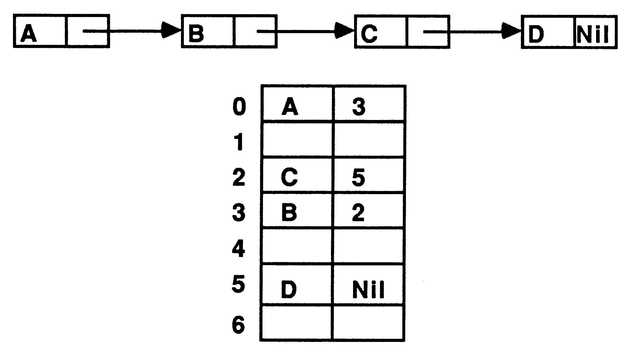
Linked lists provide a way of grouping information together and ordering information. A linear or sequential list is the simplest form of such a structure. Associated with each data item is a pointer to the next data item in the list, see figure 2. The data items are known as nodes of the list. We can implement the list by using an array of records with an extra field in each record to store the pointer to the next record. The pointers are implemented as integer indexes to the array of records.

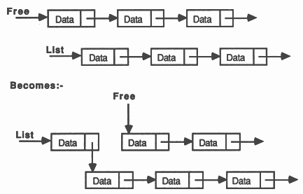
A simple example is illustrated in figure 3. Each record consists of a character and a pointer to the next node. Some of the records are not currently being used, these could be kept on a ’free list’ allowing easy location of spare space. The free records should be chained together using their pointer fields and an integer variable used to store a pointer to the first record in the chain. Abbreviations can be freely used to improve clarity throughout the code.

2.5.2 Inserting a node at the start of a list

The following procedure illustrates adding a node to the beginning of a linear linked list. It uses the structures and abbreviations declared above it.

The effect of this procedure is illustrated in figure 4. Please note the scooping of the node abbreviation. Any variable used to define the abbreviation (that is, on the right hand side of the abbreviation) may not be assigned to or input to within the scope of that abbreviation [6][1]. This allows the abbreviation to be implemented as a pointer, rather than as a copy of the variable.

Many different structures can be built up using linked lists with one or more pointers per node. A commonly used structure is a doubly linked sequential list. These have two pointers per node, one to the next node in the list and the other to the previous node. This allows removal and addition of nodes to be performed more efficiently. Non linear structures may also be built, as an example of one I shall consider trees.

2.6 Trees

2.6.1 The tree data structure with associated operations

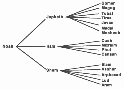
A tree is a form of directed graph, it is a natural data structure for objects that stand in a hierarchical relationship to each other. Using a tree retains the relationships between the objects and allows efficient data retrieval. As an example, figure 5 shows a biblical family tree taken from [13].

A binary tree has the following properties.

• A binary tree consists of a collection of linked nodes.
• Each node has at most two pointers.
• If two nodes are connected by a pointer from one to the other there is a ’branch’ between them.
• A tree has a node known as a root which is drawn at the top of the tree.
• Nodes may have at most two branches leading from them, nodes with no branches are called leaves.
• Each node, other than the root, must be pointed to by exactly one other node, this ensures no cycles are formed and that all nodes are connected.
• Any node, other than the root, along with all nodes and branches below it is called a subtree.

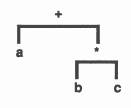
A binary tree is a natural data structure for expressing arithmetic expressions. The tree structure in figure 6 represents the expression a + b ∗ c.

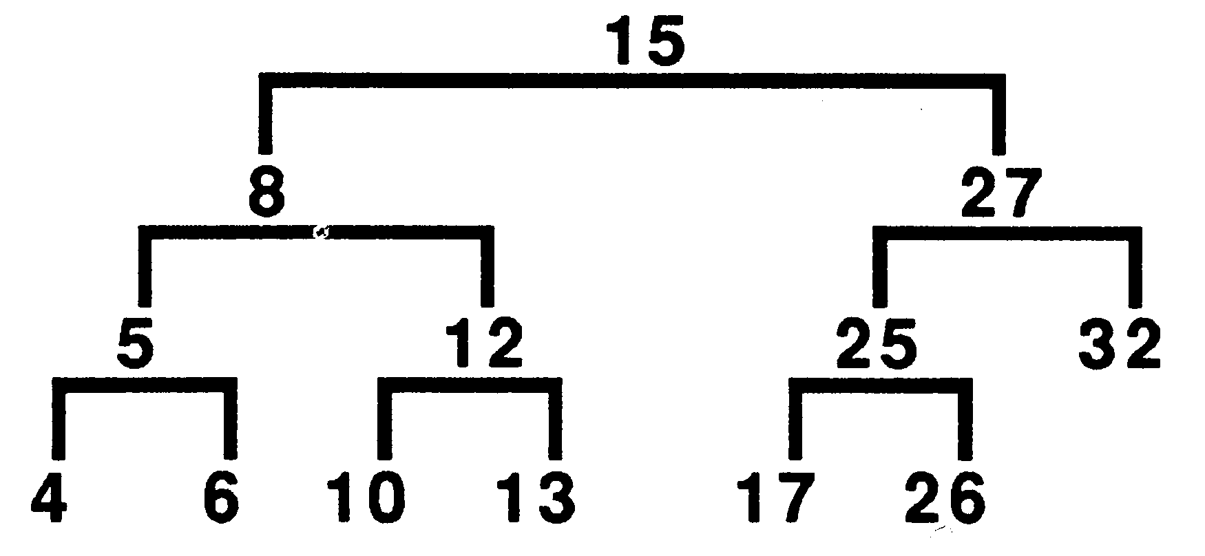
A binary search tree is empty or consists of a root with two binary search trees called the left and right subtrees. Each node contains a value known as it’s key. All the keys in the left subtree must be less than the key in the root. All the keys in the right subtree must be greater than or equal to the key in the root.

To locate a particular key start at the root and proceed to the left or right subtree by inspecting the node’s key. Trees may be forced to grow in a balanced fashion such that n elements may be stored in a tree with height as little as log n. Therefore a search among n objects can take as few as log n comparisons.

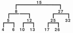
Figure 7 shows an example of a search tree. The number displayed at each node is an integer key. In the example the node with key value 12 needs two branches to reach it. In an ordered linked list it would require five branches, see figure 8. It takes an average of log2 n branches to reach a required node, as opposed to n∕2 in a sequential linear list, where n is the number of nodes.

2.6.2 Occam implementation

As an example, I include a procedure to search a tree. The procedure uses the tree definitions listed.

The data structures discussed consist of an area of store along with associated variables such as stack pointers, pointers to the head and tail of a queue, and pointers to the start of lists and roots of trees. These variables could be stored in the array used for the data structure they reference. For instance, the first element of an array implementing a stack could be reserved for the stack pointer, the associated subroutines would access this element rather than a free variable. This would simplify passing data structures between concurrent processes.

3 Recursion

3.1 Recursive functions in mathematics

A recursive function in mathematics is a function defined for every case n, such that the case for n = 1 is given and it is shown how any case after the first is obtained from the preceding one. A monadic recursive function contains only one recursive call on the function itself, a dyadic recursive function contains two such calls.

For example,

3.2 Recursive functions and procedures in computer programming

In computer programming, a recursive function or procedure uses itself as a function or procedure respectively. Recursion makes some programs more readable and many complex algorithms can be written extremely elegantly using recursion. To implement recursion directly needs dynamic allocation of space and so many programming languages do not allow a subroutine to be defined in terms of itself, e.g. in Fortran. The problem that recursion involves is the storage and retrieval of the variables in the subroutine. If the subroutine is called again the new values of the variables will over-write the values in the last call. Therefore, recursive subroutines must store the values that will need to be retrieved.

For example consider the following factorial function written in C.

Recursive subroutines can be written in any language by explicitly programming the saving and restoring of variables.

4 Transforming recursion to iteration

4.1 Monadic tail recursive definitions

The problem that faces us is how to transform a recursive definition to an iterative program. Many recursive algorithms map neatly and efficiently to simple iterative programs, not necessarily using a stack. The type I shall briefly consider here are expressible as monadic recursive definitions of the following type [5]:

Where a(x), b(x) and d(x) are directly computable functions of x, c(x) is a directly computable function of x with a boolean value, and ∗ represents a binary operation.

These recursive definitions are known as tail recursive because the recursive call occurs as the last statement in the definition. This group of algorithms map trivially to iteration. The equivalent iterative program for the definition above is described in the following section of pseudo code.

Where StackEmpty() is a function that returns TRUE if the stack is empty, FALSE otherwise. This code uses a stack and has two WHILE loops. The first loop calculates successive values of x until the base condition is reached. The second loop uses those values to generate the result. Two temporary variables, nextx and subresult, have been introduced.

If the function b(x) has an inverse, h = b⁻¹(x), then we do not need to use a stack as the successive values of x may be calculated from the base condition:

This produces more concise code but may incur performance loss. See [3] for discussion of performance maximisation in occam.

If c(x) is equivalent to x = x₀, with x₀ a constant, then the recursive definition will be of the following form:

where a is a constant, the value of a(x₀), and h = b⁻¹(x). This can be expressed as an iterative program using no stack and only one WHILE loop.

4.2 An example

As a trivial example, consider the factorial procedure mentioned above. The equivalent recursive definition is:

and the equivalent iterative pseudo code is:

which can be reduced by replacing subresult by result:

4.3 Dyadic and non-tall recursive definitions

Dyadic and non-tail recursive definitions are, in general, not trivial to transform to iterative programs. J. Arsac has done some interesting work in this area [5][7]; his method is summarized below.

First change any local variables and formal parameters into global variables. Next divide up the recursive program into a set of processes. Each process must be named and may include calls to processes. One or more of these processes will be recursive.

The processes are then ’regularized’ by ensuring that each process terminates with a call to a process, that each process is described only once, except the halting process which need not be described, and that every call to a process occurs in a terminal position.

These processes are then combined into an iterative procedure, simplifying at each stage. The three rules that govern the combining are as follows.

Substitution

A call to a process may be replaced by the body of that process.

Identification

If two processes X and Y differ only by the occurrences of the names X and Y then replace Y by X everywhere and remove the process Y.

Recursion

Removal The occurrences of recursion will be tail recursive because we are dealing with regular processes - every call to a process occurs in a terminal position. If the process is of the form X=f(X,Y), that is X depends only on X and Y, then the process may be replaced by a new non recursive process, by enclosing the recursive definition in a WHILE loop, replacing X by a null statement and Y by an exit statement, and putting Y after the loop.

5 Two approaches to recursion in occam

Unfortunately, many recursive definitions do not fall into the form described in the previous section. Other algorithms must therefore be developed, the form that they take will depend upon the nature of the problem being transformed. I shall now discuss two such methods.

5.1 The pipeline method

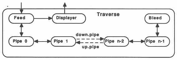
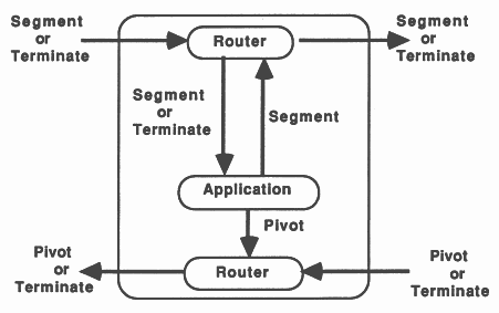
This method implements recursion using a pipeline of communicating processes. The pipeline consists of a Feed procedure to feed the initial parameters to the pipe, the nodes of the pipe which are identical processes implementing the recursive definition, and a Bleed procedure to receive results from the pipeline, see figure 9.

This is implemented in occam using a replicated PAR structure. The replicator index is used to index arrays of channels thus providing communication between the nodes of the pipe. The base and count defining the bounds of the replicator index must be compile time constants. The following example shows a bi-directional pipeline.

Each time a recursive call is encountered another node in the pipeline is ’activated’ by being passed parameters to process. When the recursive procedure is initially called the parameters are passed to the first node in the pipeline.

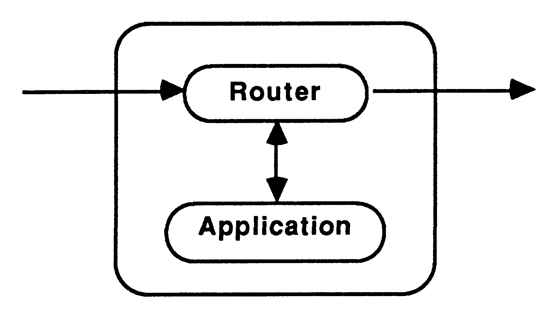
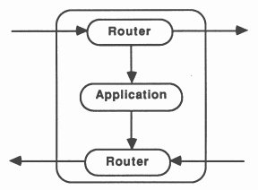
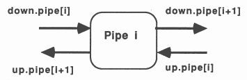
The nodes of the pipeline will take one of three forms, the application only (i.e the recursive definition), the application with one router (see figure 10), or the application with two routers, see figure 11.

On the transputer, routers should be run at high priority with the application at low priority [3]. Thus, when data is received to be routed to a waiting node, the routing process doesn’t need to wait for the application process to finish before passing on the data. The routers would receive data from further up the pipe, and send the data either to the application process, if it is waiting for data, or to the next node in the pipeline. Routers would also pass results back up the pipe to Feed or on down the pipe to Bleed. Using two routers allows data to be passed along the pipe via the shortest route.

Dyadic recursive definitions would send parameters to be processed down the pipe until an available node is reached. Thus, each router would keep a boolean variable to show whether its respective application process was busy, indeed any number of recursive calls in the definition could be catered for using this method. Monadic recursive definitions will always use the next node in the pipeline and so they may not need a router. If the application does not need to wait for the results to be returned from the recursive call before continuing to process, a router allows the communication to continue in parallel with the computation.

Consider the two mutually recursive procedures below.

Each of the procedures calls the other, i.e X calls Y which calls X which calls Y... This could be implemented by using a pipeline with nodes consisting of the procedures alternating with each other, see figure 12.

Suitable routers and tagged protocols to control parameter passing should be used for variations on this theme, for instance, mutual recursion combined with self recursion.

The number of nodes in the pipeline must cater for the worst case. This may involve a large amount of redundancy. An alternative would be to have less then the worst case of nodes in the pipeline and use farming methods to ensure no overflow occurs. A process to control the flow of data into the pipe would be used to implement the farming, buffering the data to be processed and only sending data as nodes become available [1][8]. All nodes must, of course, be made to terminate, not just those that were used for the computation. The usual method of termination is to propagate a termination signal down the length of the pipeline. This can be implemented by using a tagged protocol.

A suitable application for the pipeline approach would be highly computationally intensive with a relatively small amount of communication between the processes.

5.2 The stack method

This method implements recursion by explicitly storing variables on a stack. The variables that need to be stored are any local variables and any parameters for each recursive call. These should be changed into global variables for the iterative procedure, effectively removing parameters to the procedure. The basic method to transform the recursive algorithm to an iterative program is as follows.

Push the relevant variables onto the stack before each recursive call and Pop them off again on return from that call. For example, a recursive call to F of the form F (g (x)) will be changed to:

If the function g has an inverse, h, the parameter need not be stored on the stack as the old value of x can be recomputed on return from the recursive call.

If we are now to remove the recursive calls and surround the procedure with a WHILE loop which terminates when the stack is empty we will need to ensure that we continue processing at the correct point after each re-entry of the loop. The definition should now be of the following form.

Where a, b, c and d are sequences of statements and bool is a boolean expression.

Thus after the first recursive call processing should continue with c, after the last call it should continue with d and on initial entry processing should start with b. The correct flow of control is implemented by storing an action field on the stack and selecting the correct sequence of statements in the following way,

Usually, the push/pop operations for the action and the variables that need to be stored would be combined. Obviously, meaningful names should be used for the action specifiers.

6 Two recursion examples

In order to demonstrate implementation of recursion in occam I will work through two examples using both the stack and the pipeline approaches. The examples chosen are two ’classic’ uses of recursion, traversing a sorted tree and the sorting algorithm known as quicksort [9][10].

Neither of these examples are particularly suitable to the pipeline approach, they have been chosen for the sake of simplicity.

6.1 Recursive tree traversal

6.1.1 The recursive algorithm

The procedure traverses a tree implementing recursion using a stack. The equivalent recursive algorithm is show below.

6.1.2 The stack implementation

The recursive definition has no local variables and the recursive call has only one parameter, a pointer to the current node of the tree. Therefore, each record in the stack consists of two fields, an action field and a pointer field. The pointer contains an index to the array that implements the tree structure, it points to a particular node in the tree. The action takes one of three forms: DownLeft, DownRight and Done. These signify that the left or right subtree of the node pointed to should be traversed or that the tree has been fully traversed and processing should terminate.

The following pseudo code describes the algorithm used.

Thus, each node traversed causes a record to be pushed on to the stack, implementing the recursive call to traverse the right subtree. The tail recursive call to traverse the left subtree is implemented by the while loop.

The tree is implemented in occam with an array of the following form:

The stack and its operations are implemented in the following way:

And, finally, the code for the procedure is given below.

6.1.3 The pipeline implementation

The procedure traverses a sorted tree using a pipeline of communicating parallel processes to implement recursion. The equivalent recursive algorithm is shown in section 6.1.1.

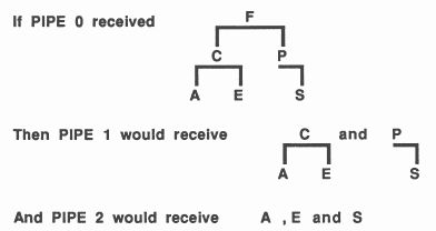
Each node in the pipeline is passed a pointer to a subtree of the global tree. Each level in the tree corresponds to a level of recursion in the algorithm shown above. Thus each node in the pipeline performs the same actions on a different level of the tree. The maximum number of levels in the tree must be known before hand, the pipeline will need that many nodes.

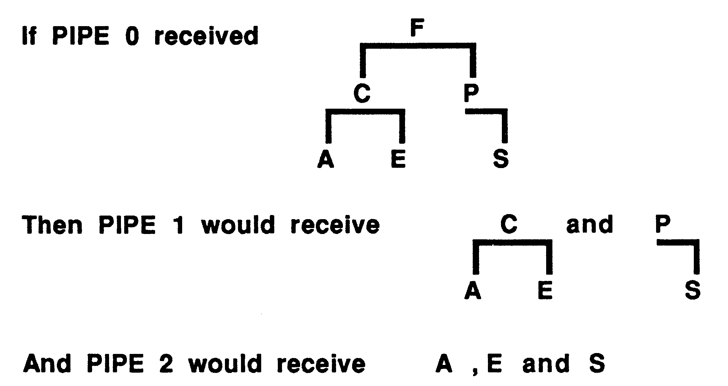
The first node in the pipeline receives a pointer to the root of the tree and passes the root’s left subtree to the next node in the pipeline. When that subtree has been processed it prints the value at the root of the tree and then passes it’s right subtree to the next node in the pipeline. See figure 13 for an example.

Figure 14 shows the processes that make up the traversal and the communication channels between them. The processes run in parallel, with the order of the characters maintained by communication interlock between the processes.

Feed:

Sends the root of the tree to the head of the pipeline and passes data for printing to the displayer.

Bleed:

Deals with the last level in the tree, which consists of NILs.

down pipe:

Passes subtrees deeper into the pipe.

up pipe:

Passes data for printing back to root and notifies higher levels when subtrees have been processed.

The following code shows the structure used in occam to initiate bleed, feed, display and the pipeline. The pipeline is created using a replicated PAR with the channels indexed by the replicator index.

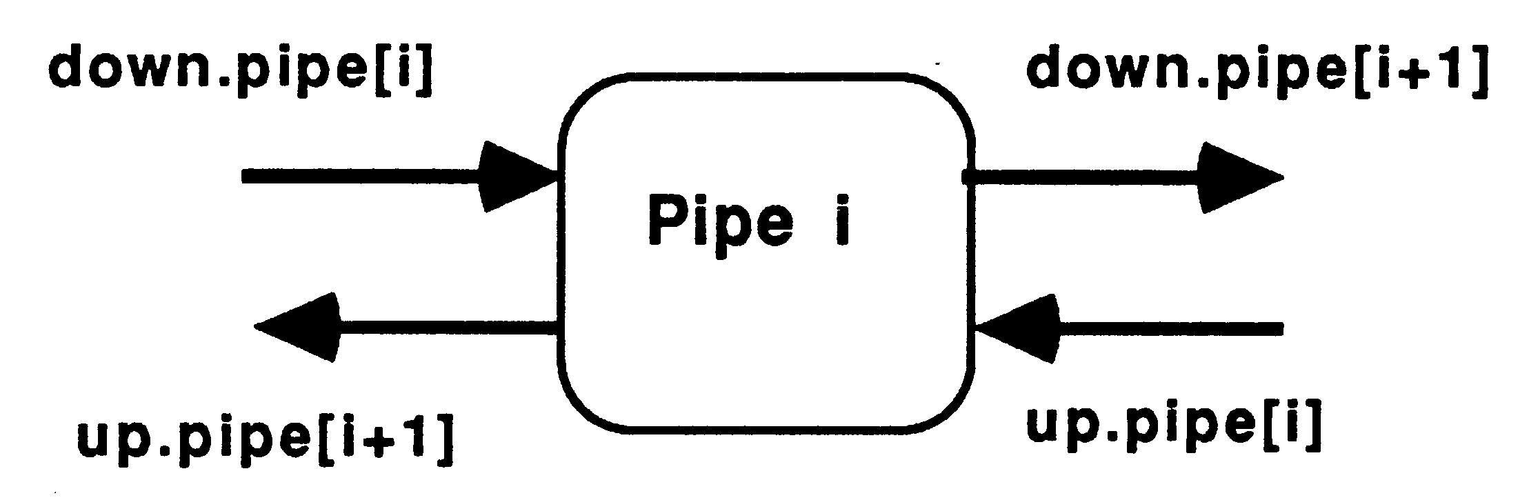
Figure 15 shows the channels that each node in the pipe has access to, and the pseudo code below describes the algorithm used to implement each node.

When Feed receives a NIL from the first node in the pipeline the whole tree has been traversed. Feed then sends a termination signal to the displayer and to PIPE[0] which propagates down the rest of the pipe. Finally, the last node in the pipeline passes the termination signal to Bleed.

6.2 A recursive quicksort

6.2.1 The quicksort algorithm

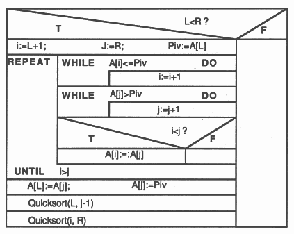
The quicksort, or partition exchange, algorithm sorts a string. It finds the correct position of the first element in the string. This element is called the pivot. It places the pivot after all elements less than or equal to it and before all elements greater than it. This partitions the string into the positioned pivot and the substrings before and after the pivot, which are then quicksorted recursively.

The following example demonstrates the method.

Where square brackets represent substrings still to be sorted. Thus the sort replaces the sorting of n items with sorting two lists of less than n items. Figure 16 gives a Nassi-Shneiderman diagram [12] of the algorithm which sorts the contents of the array A[L..R], where A[R+1] >= any A[L..R] .

6.2.2 The stack implementation

The recursive definition has two tail recursive calls with substrings as parameters. These can be stored on the stack as two integers, left and right pointers to delimit the substring within the initial string to be sorted. As both the calls are tail recursive, they have the same entry point and so only two actions are needed - Done and Sort. The records of the stack therefore consist of two integer pointers to the array holding the string and an integer action field. The following pseudo code describes the algorithm used.

6.2.3 The pipeline implementation

The quicksort algorithm is described in section 6.2.1 above. Each node of the pipe will consist of the sorting procedure along with two routers, see figure 11. The recursive definition has two tail recursive calls, one of which may easily be converted to iteration by changing the left and right limits of the current substring and enclosing the procedure in a WHILE loop. Thus any left hand partitions are sorted by the same node and any right hand partitions are passed down the pipeline to the next non-busy node.

When the position of a pivot is found, it and an integer pointer to it’s position in the original string are passed down to the Feed procedure. When all the characters have been positioned Feed sends a termination signal down the pipeline. This is propagated down to Bleed then back up to Feed again.

The pipeline is implemented as for the bi-directional pipeline in section 5.1. The nodes of the pipe are described in the pseudo code below. See figure 17 for a diagram of the nodes.

The Feed and Bleed procedures are described by the following pseudo code.

References