Contents

1 Introduction - background to the GPS

GPS arose from early experimental American military programs interested in clock stability and relativity, such as the ”Timation” program in the 70’s. The specifications of the prototype system became public in 1978, with a full issue of the (American) Institute of Navigation Journal being dedicated to the subject.

It is based on the concept that if you know your exact range from three known positions, you can calculate your position in three dimensions. The range is determined by the propagation delay of the signals from the satellites, which assumes you knew when they were transmitted. Short of carrying an atomic clock in every receiver, this is solved by using a fourth satellite, and using the redundancy in the position equations to solve for time also. Whilst earlier satellite navigation systems such as TRANSIT used doppler shift as the measuring domain, GPS uses propagation delay.

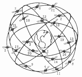
Contrary to popular opinion, the satellites are NOT geo-stationary. They are in a inclined orbit that takes them over any point in their ground track approximately every 12 hours. Figure 1 shows that geo-stationary satellites cannot provide three dimensional positions, nor latitude accuracy near the equator, nor any coverage of the polar regions.

There are currently six operational satellites, so coverage is severely limited. This is largely due to delays with the NASA shuttle. It is anticipated that the full constellation will be in service by 1995, with useful coverage of the UK by mid 1990.

1.1 Space Segment

The system consists of eighteen operational satellites in six orbits, with a spare satellite also available in each of the six orbits. This is a relatively recent change from the original spec, which had the satellites divided over only three orbits. The spec may change again, as the current orbits, being almost synchronous with the earths rotation, albeit at twice the frequency, suffer cumulative orbit disturbance due to the sun and solar flux. Desynchronising them would give a more stable orbit with less need for firing the jets.

The satellites all transmit on the same frequency using a spread-spectrum technique. To spread the spectrum of the signal, inherently only 100 Hz wide, it is multiplied by a code-sequence known as a Gold code after its inventor. As the chip-rate of the code is 1.023 MHz, this results in the transmitted signal having a bandwidth of around 2 MHz, with a very low power density (-163dBW). This is far below atmospheric and front-end noise.

Each satellite has a unique code, so when the signal is descrambled, the energy from a particular satellite only can be extracted.

1.2 Command Segment

The satellites transmit a carrier modulated by the Gold code and also by useful data needed in the receiver to work out both the satellite position and the user position. Coefficients are transmitted that allow the exact position of the satellite to be calculated, and also measured values of the ionospheric propagation characteristics. This data is uplinked to the satellites by the ground stations around the world, after considerable computation to perform curve fitting such that the new parameters can remain valid for at least four hours, even though they are uploaded every two hours. The ground stations are at Ascension Island, Diego Garcia, Kwagale, Hawai, controlled from the master station at Falcon Air Force Base, Colorado. These give global coverage, so satellites are never out of sight of a control station for more than the two hour uplink interval.

The data sent by a satellite consists of detailed information about its own orbit and transmission parameters, and at a slower rate, less detailed information about all the other satellites. This latter data, known as the almanac, is useful as it allows acquisition of satellites after the first to be directed at the correct code, and also the correct doppler offset.

1.3 User Segment

The user has to receive the off-air signal, from at least four satellites, and descramble it to determine both the timing information and the downloaded data.

To receive the signal, he must use an aerial that can see almost an entire hemisphere. The spec asks for down to 5 degrees above the horizon.

In order to descramble it, he must generate a copy of the satellite code and multiply the incoming signal by it, at the correct offset to allow for propagation delay, which must be found empirically. This then gathers the energy from the required satellite, whilst spreading out the noise, and the other satellites even further.

Finally he must use the offset and data to calculate first the satellites, and then his own, position. For the satellites, this is largely a case of plugging the downloaded coefficients into given equations, but there is one small calculation that must be performed iteratively. For the user position, a matrix of four simultaneous equations must be solved, and it is most convenient to handle this iteratively.

2 The traditional approach

The traditional approach consists of a dual conversion superhet front-end, using coherent local oscillator and intermediate frequencies, then four or five hardware signal processing paths that each deal with one satellite, feeding their output to a processor which performs the calculations and handles the user interface.

2.1 RF front end

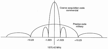
The RF front end must take the incoming signal at 1575.42 MHz, 2 MHz wide, with a received power of -163dB, and amplify it and down convert it to a convenient frequency. The spectrum is shown in Figure 2. The wider curve is the military signal, whose code is secret, so we cannot unscramble it. The desired signal is the Coarse Acquisition (C/A) code, which forms the central peak.

It is usual to use a first IF of 100-200 MHz, in order that the front end image frequency is easily eliminated. Some systems only use the single IF, but running phased locked loops at these frequencies is inconvenient, so most use a second down conversion stage, to a frequency of 5-20 MHz.

All frequencies used in the satellite are a multiple of the 1.023 MHz basic chipping rate, so it is convenient to use other multiples for IFs and local oscillators. Thus the carrier is 1540 * 1.023 MHz. If the first IF is to be 120 * 1.023 MHz, ie 122.76 MHz, then the LO is 1420 * 1.023 MHz. Another favorite is 160 * 1.023, ie 163.68 MHz.

Choosing such multiples means that all local signals can be generated synchronously from the same chain, and thus be completely free of undesired beat frequencies. The actual incoming carrier is of course not exactly on frequency, due to doppler shift from the fast moving satellite.

2.2 Hardware signal processing loops

The signal tracking hardware is the most expensive section of the receiver. In early sets, it consisted of a satellite code generator, a very narrow filter, and a phase locked loop, with the offset of the code generator and the frequency of the PLL being swept empirically until the signal was found.

The signal processing consisted of two mixing (or multiplying) stages. The first multiplied the incoming signal by the locally generated satellite code. This does not alter the centre frequency, but it does, when synchronised, pull all the satellite energy from the 2MHz wide signal into a single narrow carrier.

The output of the PLL was used in a down conversion mixer to make the carrier, now only 100Hz wide, hit the passband of the filter. The filter had to be very narrow in order to achieve the required noise performance, but due to doppler shift, it would then miss the carrier without such tracking.

In order that the hardware could detect such a signal, the PLL normally runs at twice the final carrier frequency, so that the BPSK modulation on the carrier does not affect it. A divide by two and an exclusive-OR gate can then extract the download data stream from the satellite.

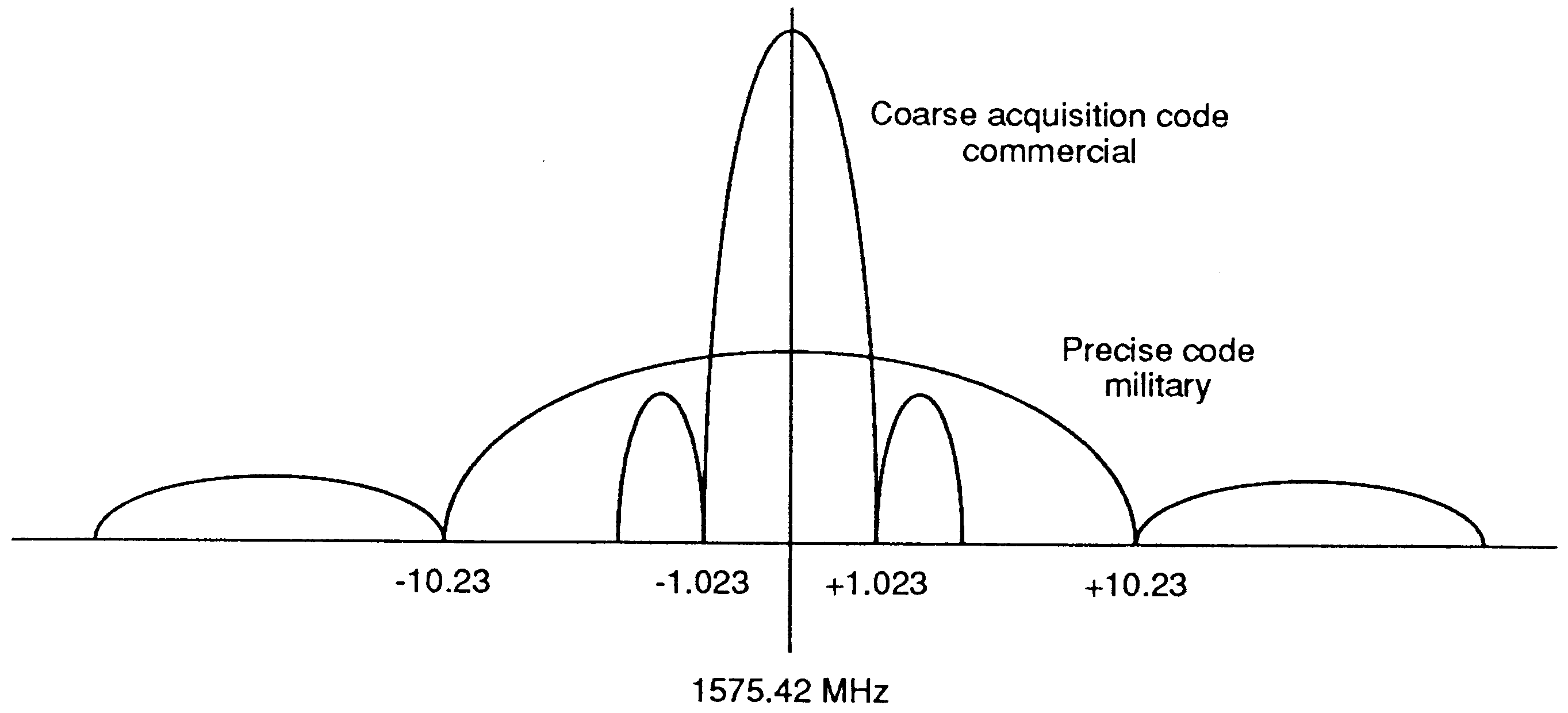
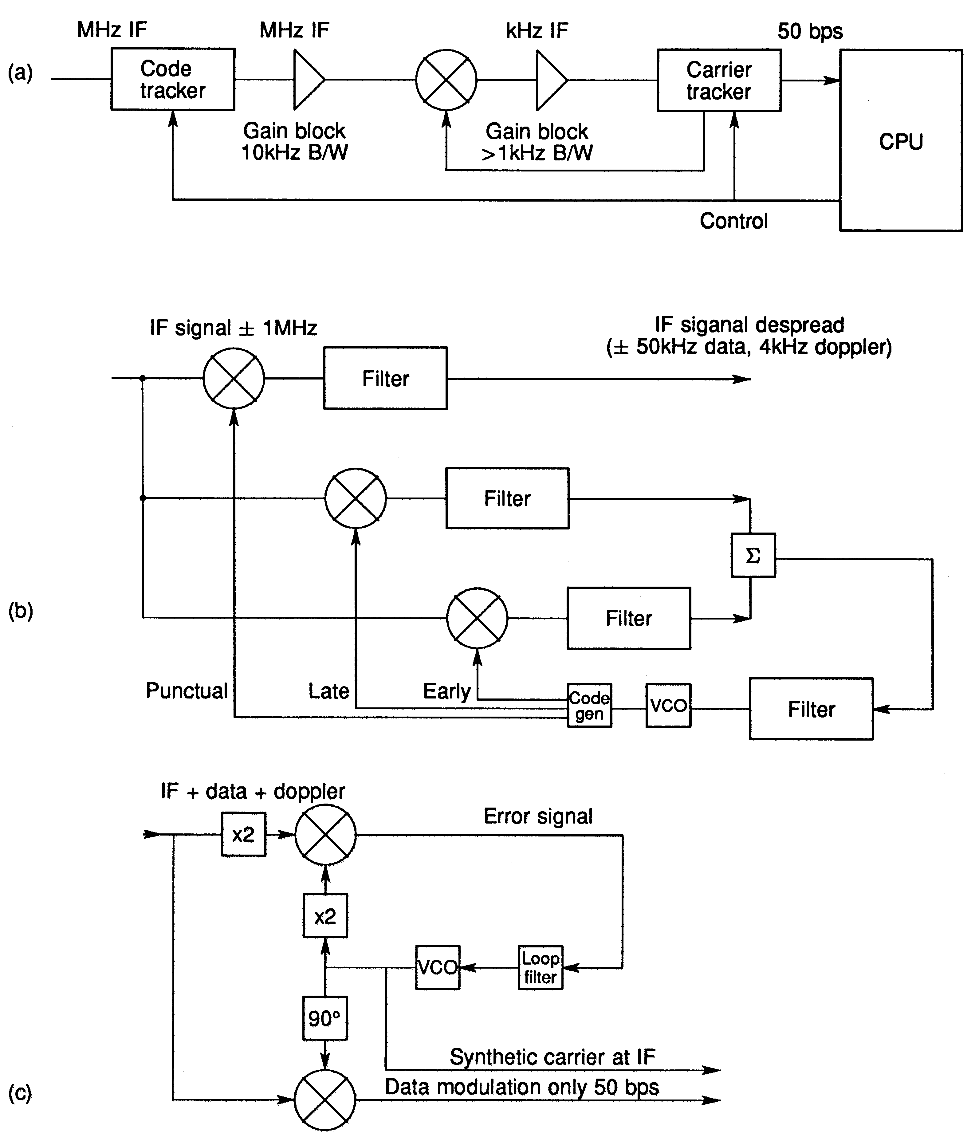
The traditional hardware receivers require one of these hardware tracking channels per satellite, Figure 3 (a). Sections (b) and (c) are a traditional code tracking loop and a hardware tracking loop respectively. (Taken from [4].)

Such hardware could, in 1980, use a card per satellite. However rapidly the use of higher levels of integration, or even custom chips, allowed it to be reduced, but it still remained the major section of the hardware.

2.3 Processor

In the earliest systems, the satellite tracking was almost entirely autonomous, with the processor interested in only the code generator offset and the down load data from each of the four or five channels. As faster micros became available. the micro was used inside the hardware loop to command the code generator, and command the PLL frequency.

The main task, however, was to perform the mathematics to calculate the position, and to monitor the keyboard and drive the display.

As the hardware tracking loops became more integrated, they ceased to be autonomous, so the micro workload grew, especially on receivers designed for high-dynamics vehicles, where predicting the doppler shift becomes a problem.

Despite the rapid increase in microprocessor performance, all the signal processing was still done in the hardware tracking channels, as the micro could not historically keep up with the speed demands.

3 Why change?.. the problems

It was decided to design a hand held receiver. That means low chip count for size and for power consumption. It also means rapid satellite acquisition time, both for convenience (ones arm starts to ache after a very few seconds of holding something at arms length), and for battery life.

Thus the problem area to be attacked was the hardware signal processing. This used a large number of chips, as the custom ASIC approach was not open to me, and thus also space and power. It also is the section that determines the acquisition time... and the traditional approach takes an average of 44 seconds to acquire a satellite, worst case of double that. The reason for this long time is that it must search thru a large number of frequency domains( say 10), and a large number of code offsets(2046), resulting in 20000 trials, each requiring the lock up time of the PLL.

4 What the transputer brings to the party

The transputer is a very high-speed general purpose processor, with on chip serial communications that can transfer up to 1.8Mbytes per second on each of 8 links (4 in, 4 out). The communications is autonomous from the processor, which only authorises the communication at a cost of about 1 us per message, no matter what the message length.

So the transputer can perform i/o operations concurrently with the main processing. Even more significant is the speed of the processing... the simple maths operations such as ADD or XOR needed for this type of signal processing take 50 or 100 nanoseconds.

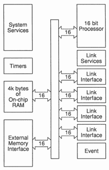
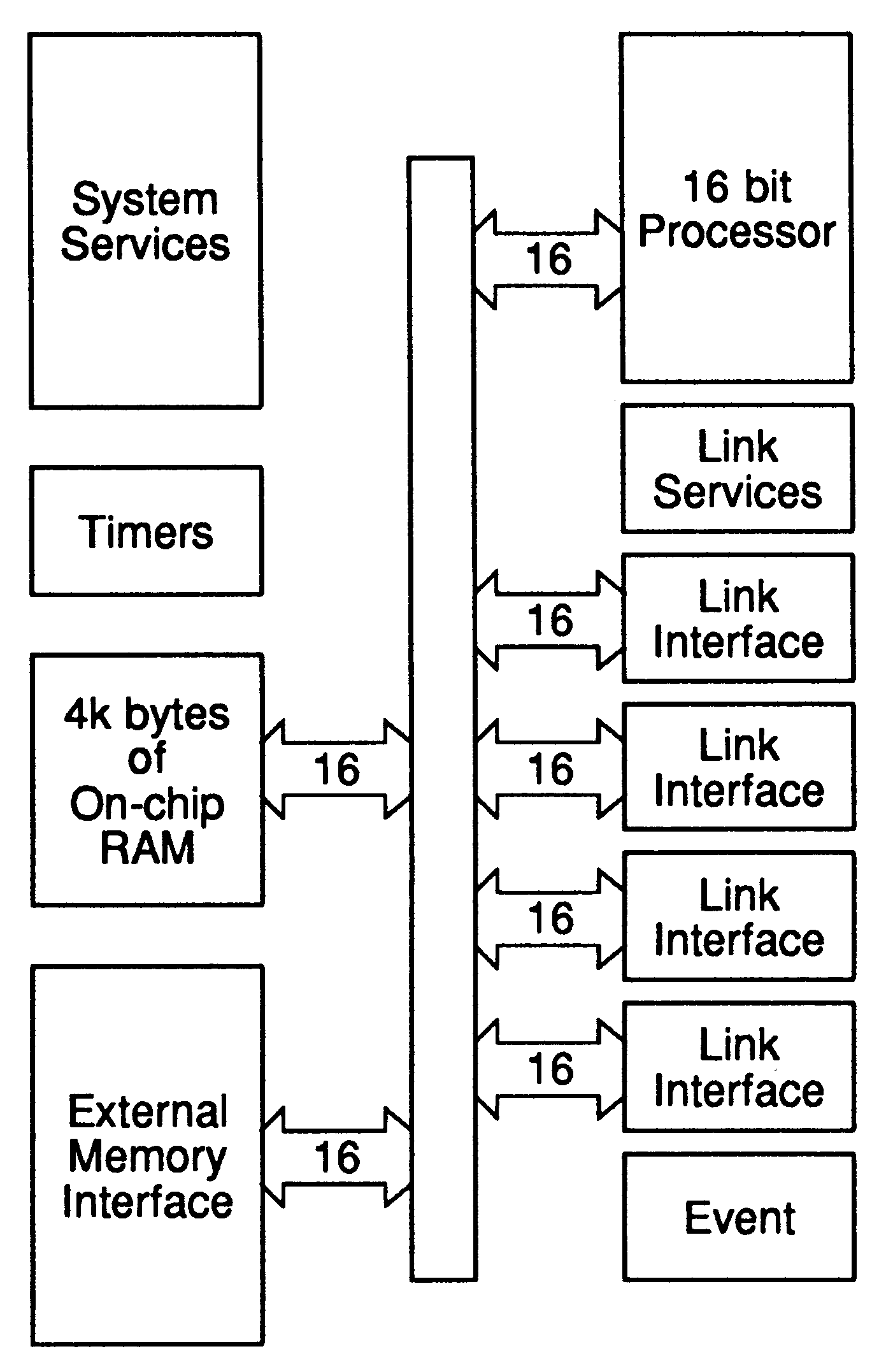
In order to allow such speeds of I/O and computation, the transputer provides 4Kbytes of static RAM on chip (Figure 4). Being on chip it cycles in 50ns on the 20MHz parts, avoiding the problems of driving pins and printed circuit tracks to external memory.

If more than 4kBytes is needed, it can be added externally, and then slow inexpensive memory can be used, as the time critical programs can be given the fast internal RAM.

The availability of a 10MIPS machine rather than the 0.5MIP micro conventionally used makes a significant difference to how the problem can be approached. Suddenly it becomes possible to handle the signal directly with the micro … and in the case of GPS, this means 5 separate signals.

Another major feature of the transputer is the hardware scheduler. Even a single transputer can handle multiple jobs at the same time. Conventional processors doing this take a large percentage of the CPU time managing the interaction between them, but in the transputer, this is performed entirely in hardware at negligible time penalty. As a result the input job, performed by the serial communications hardware, the signal processing job, and the computation/user interface job can all run simultaneously, and the CPU will switch from one to the other transparently.

5 The new approach - Software Signal Processing

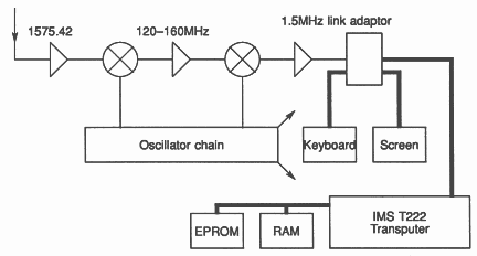
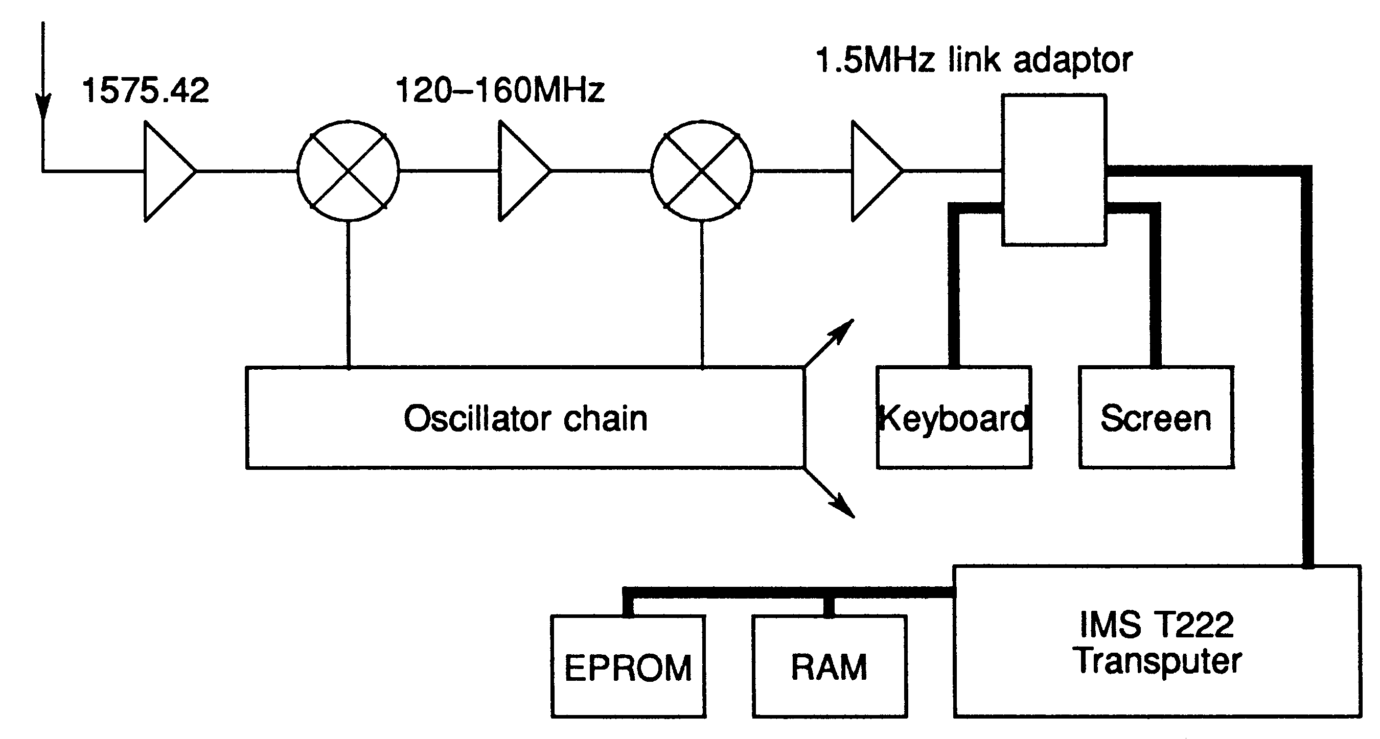
The new approach is to perform all the signal tracking in software. Essentially the same RF front end is used, but to a lower frequency of around 1.5 MHz... the lowest frequency that can conveniently handle the bandwidth. This is then fed into the transputer for processing as shown in Figure 5.

The signal has to be read in to the processor, multiplied by the locally generated code, filtered and detected. The easiest way of achieving the last two operations is to down convert to a low frequency and apply a low pass filter, then perform an FFT if the frequency is unknown, or a synchronous down conversion to DC if the frequency has already been determined. In the following sections, we will cover the approach taken for a single satellite, then later demonstrate how vast economies can be achieved when performing the work for multiple signals.

5.1 Input

To input the signal two methods were tried - an analogue to digital converter, or hard-limited one bit signals. With the former, one is severely limited in I/O bandwidth, and does not achieve a 100 per cent duty cycle. One takes a few milliseconds of off-air signal, and processes them inside 20 milliseconds, resulting in a 10 - 20 percent utilisation of the incoming signal.

With the hard limited approach, a faster sampling rate can be used without hitting I/O limits, and by devious tricks that process a word’s worth of samples (16 or 32) in a single instruction, a vast saving in processing

can be achieved. Additionally no AGC circuits are needed in the front-end.

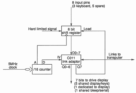
Thus the chosen design clocks a hard limited signal into a shift register, and when a byte has been collected, feeds it down a transputer link using a link adapter. This uses a link adapter plus two TTL chips (Figure 6). Because the link is attached to an autonomous DMA engine in the transputer, no CPU time is involved in input.

5.2 Code Correlation, Down Conversion

Once a buffer has been filled in the processor, the hardware scheduler wakes the cpu, which switches buffers so that the next message will go into another buffer while this one is processed. Thus the data is never copied, it is processed in situ.

The code correlation function consists of multiplying the incoming samples by a code stream which is held in memory. It is a binary stream, so is packed one sample per bit.

The down conversion operation consists of multiplying by a locally generated set of samples that represent a synthetic local oscillator. These are generated once only, at start-up, or even kept in the ROM, and are also hard limited one-bit samples. The result is then at around 4 KHz, plus or minus the doppler shift.

Because these two multiplies represent the equation

it can be seen that once the correct code offset is achieved, code*local.oscillator can be calculated once and saved, thus reducing the repetitive work in the loop. Even before the offset is found, this is valid, as an offset applied to the local oscillator only represents a phase shift, which is acceptable at this stage. Note that whilst it is imperative in the analogue world to perform the code correlate before the down conversion, to prevent the lower edge of the bandwidth going negative, there is no such restriction in the mathematical world, and hence no parentheses were used in the above equation. (occam would require them)

So the equation becomes :

which by redefining the base of code.LO becomes

Now we can remember that the signal is only one bit wide, and is packed 16 to a word on the T222 transputer. A one bit multiply is an exclusive-OR operation so assuming a group of input samples in a buffer, one could use the following code:

Note that a 16 two microsecond multiplies have been reduced to a single 100nanosecond XOR operation, a speed up of 320 times!!!. Now the loop is dominated by the loop control code, around a microsecond, and the array indexing. Both these are solved by opening the loop out in-line. This removes the loop control, and allows the transputer’s very efficient constant-index instruction to be used. Assuming a buffer of 128 samples, ie 8 16bit words, this becomes:

This code generates the same number of output samples as there were input samples, so although it has performed a huge amount of work, it has not reduced the size of the data. This can be done in the filtering operation.

5.3 Filtering

The sample stream now represents a 4 KHz carrier sampled at 2.5 or 5 MHz. For 32 bit transputers, the higher rate is used, giving increased noise performance. Either rate is far higher than required, so the samples are decimated. Additionally, in order to filter the signal, a large number of samples need to be averaged.

These two tasks can be combined, and the transputer has a very effective instruction that will perform the task for a word’s worth of samples at a time. This instruction is available directly in occam as the BITCNT predefine. By careful choice of sample rates and buffer sizes, the filter bandwidth comes out correctly in the wash... this one averages 128 samples, which represent 50 microseconds sampled at 2.5 MHz, giving a filter that has a deep null at 20KHz, but passes 0-8KHz.

Thus the following code will filter and decimate, counting the number of bits set in each word cumulatively

The same rules can be applied to speed this up as before, opening the loop, but in fact the best approach is to integrate the active line into the same open loop with the correlate/convert operation, yielding:

This code compiles into extremely efficient instructions.... it can be improved by less than 5 percent by hand coding in assembler. The improvement comes from eliminating the intermediate stores to the variable ”accumulate”, and can also be achieved in occam by combining all eight lines into one, with appropriate brackets.... however it is not proposed to demonstrate this on the printed page as it is too narrow.

The assembly code instructions for the main expression are shown below. For an explanation of the mnemonics, see [2] and [3].

On a T425-20, execution time is 2.2μs per 32 samples. With overheads, this becomes 327μs per 5000 samples.

This combined code has now achieved a single sample representing 50 microseconds of off-air signal, and it has less than 20 microseconds of CPU time to do it. All future work will be done on these slow samples, so absorbs very little CPU time, as it runs only 1/128 as often.

5.4 Detection - Coarse FFT

In acquisition mode, we need to look at the output of processing using a particular code offset to determine whether a signal has been found. If the code offset is incorrect, we will be unable to find a signal.

Thus we continue in the fashion described above until sufficient slow samples have been built up.... at this stage, 16. We then perform an FFT on these samples, which will show the energy in each 1.25KHz band from zero to 20 KHz. We scan the output in the lowest 8 bands, and if it exceeds a predetermined threshold, we have found the satellite code offset and can stop searching. Otherwise, the processing repeats at a different code offset. The coarse 16 point FFT takes around two milliseconds.... and only represents one millisecond of input data, so is not feasible for a 100 percent duty cycle system after acquisition, so now having determined the code offset, we concentrate on determining the doppler frequency accurately.

5.5 Detection - Fine FFT

The input and processing system is then allowed to run for a longer period at the offset thus found. When 1024 low-frequency samples have been accumulated, an FFT is run on these, giving a frequency resolution of about 20 Hz. Thus a new low frequency local oscillator stream can be generated, which when multiplied by future incoming LF samples, will directly convert them down to base band DC.

5.6 Detection - Convolution

Future incoming low-frequency sample streams are multiplied by the new synthetic stream, yielding the down load data from the satellite. This new final down conversion needs to be performed in phase and quadrature, in order that gradual phase drift caused by slight error in the synthetic carrier frequency can be monitored, and thus not interpreted as data, and also so that the need to correct the synthetic carrier periodically can be detected. The maximum rate of change is about 2KHz per hour, or 33 Hz per minute, so a new carrier is needed every 40 seconds or so... so rare that it does not impact CPU utilisation significantly.

The sample stream on which the convolution is performed can be analogue, ie numbers in the range 0-127, or it can be hard limited and packed as it is created. This latter case costs some noise performance, but works well for the single satellite case, and takes negligible CPU time as the synthetic stream can also be limited and the operations performed a word at a time as before. However for ultimate performance, it can be done explicitly with full word values, as there will only be around twenty points per millisecond to be handled. In this case it takes about two percent of the CPU.

6 Achievements so far - now more satellites

Thus we have shown how we can acquire one satellite, taking some 36 percent of the CPU in the high-speed signal processing and some two percent in the low frequency processing. We need to track four satellites, and ideally a fifth to allow a clean handover when one goes below the horizon, so either we accept a less than 100 percent duty cycle, we add more processors, or we think up some tricks.

Reducing the duty cycle makes synchronous operation difficult, makes carrier phase tracking difficult, and degrades the noise performance. Adding processors is easy with the transputer.. they simply bolt together with no additional hardware or software, but the lower end of the market, this may not be economic. For high performance military systems, this would be the approach to take.

The clever tricks approach seems to be most appropriate. The most productive of these is to avoid having to perform the high-speed signal processing separately for each satellite, but to do it once for them all.

There are two approaches to this. One is to square the incoming signal. This automatically multiplies the code and signal by themselves, resulting in a term that is signal squared, with the code removed. However this removes all code timing information, and tracking must be done from the the carrier phase. Such systems are very hard to initialise, and could not use the hard limited approach, as squaring a hard limited signal has no meaningful effect.

The second approach is to use a composite code method, where a synthetic code is created that is the best approximation to all four or five codes required on a per bit basis. Initially this code is created with no offset between the codes, and is run through the sample stream to find all the satellites. Knowing their offsets, a new composite code is created so that the codes are correctly offset, and a single pass over the data will pull out the signal for all four satellites. Thus the same 36 percent of the CPU time will do the work for all the satellites, and the same acquisition effort likewise.

The low frequency work must still be done separately, but this means that the 2 percent becomes 8/10 for 4/5 satellites, or still negligible if one performs it on a single bit basis.

Just as the synthetic carrier frequency will drift due to changes in the doppler shift, the code offsets will change due to the satellites movement. They will reduce for ascending (approaching) satellites, and increase for descending ones. The maximum rate of change, however, is about one chip every 1.5 seconds, [4], so the creation of a new stream every half second would suffice, again absorbing negligible CPU time. Once the first position fix has been obtained, all these changes can be predicted, and additionally they can be monitored .. this one by dithering the offset by one incoming sample and establishing whether the advanced or retarded signal is stronger for each satellite, allowing fine tuning of the prediction.

7 Position Calculations

We now have a system that can acquire and track the signal from five satellites continuously with a 100 percent duty cycle, with 3 to 5 MIPS of CPU resource still available for position calculation, the remainder having been used by the signal processing.

The satellite position calculation requires simple calculations plugging in the coefficients down loaded from the satellite, and this takes less than two milliseconds of CPU time. The equations are given in the GPS spec [1].

The user position calculation is a solution to the four equations

for i = 1 to 4, where Range is the distance from satellite to receiver, calculated from the propagation delay assuming a perfect receiver clock, c is the speed of light, t is the user clock error (unknown), XYZ is the user position (unknown) and XYZi is the position of satellite i.

The user clock error becomes the fourth unknown, with XYZ, to be solved for. Note that the first result will not be perfect, as the satellite positions were calculated with respect to time, and the time used was ”wrong”. However successive calculations will yield progressively more accurate results for t, and thus for XYZi, and thus for XYZ.

The user does not need a position update more frequently than once every five or ten seconds, so it is usual to put a filter on the data that averages over such a period before running the position calculation. Such a filter can also allow for short outages of a satellite signal caused by local obstructions such as tall buildings. However on a portable set, a repetitive display is probably unnecessary... the above equations could be solved iteratively until the results stabilised, and then the complete set turned off except for the display, in order to conserve power.

A marine (yacht) receiver would have an additional suite of software to provide data such as average course and speed, to give distance, bearing and estimated time of arrival at the next waypoint, to follow a route or sailplan through a pre-selected group of waypoints; and to raise various alarms when off course. It would also provide outputs to control an autopilot. All this software has been written for the transputer based navigation system... it is a lot of code, but executes relatively rarely, so does not impact on the CPU time.

8 Mechanical Details, Display and Keyboard

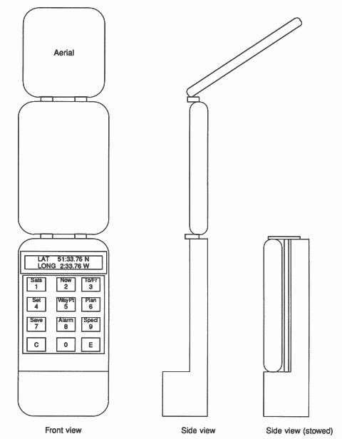
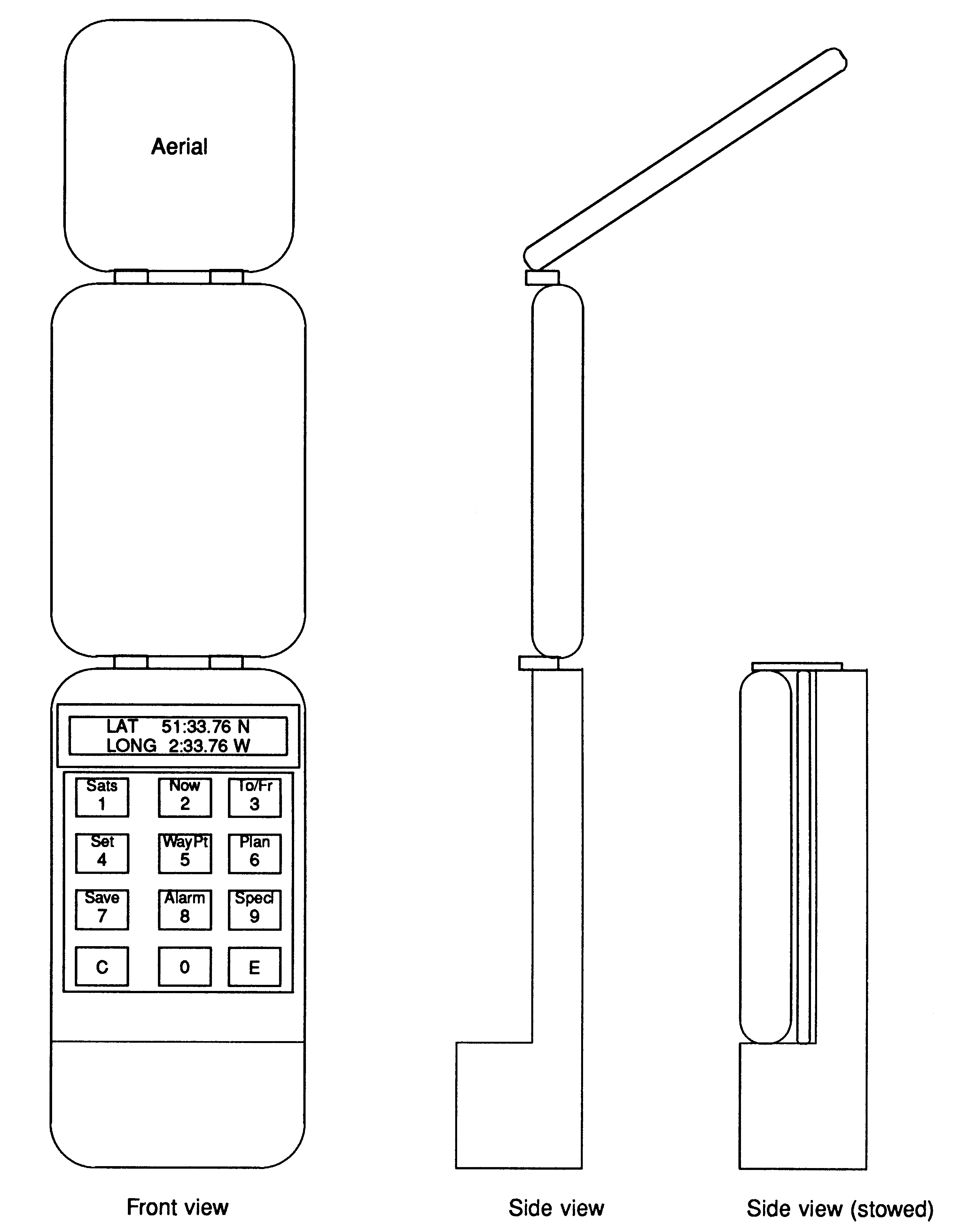
The display of a handheld version need only be a position, either in latitude and longitude or in local coordinates such as National Grid Reference. However my implementation allows for the handheld to be used on boat, so includes the larger display and a keyboard for mode selection and waypoint entry. The prototype uses a display with two lines of forty characters, organised such that it can be exchanged for a 4 x 20 character version. These have compatible interfaces, and the latter allows the face of the unit to be 100mm wide by 170mm high, suitable for a hand-held pocket set.

The Link Adapter described above for inputting the off-air signal also provides 8 output pins. These are use to drive the display module, and to strobe the keyboard and operate a bleeper to acknowledge key depressions. The shift register used to capture input samples also has a parallel input, and this is activated to read the keyboard as necessary. Thus no additional hardware is needed. This entails some slightly complex software to share the transputer link, but is worthwhile on a portable. On the marine version a second link adapter for the user functions has been used. This allows a clean separation of the software, and also makes a separate control head for the charthouse, the cockpit and the flying bridge very economic extensions.

The simple handheld version would have the transputer, three 28 pin chips and 4 TTL packages. If the navigating functions are included, it would use more memory, expanding to 5 28pin chips. The processor board is the same size as the keyboard,about 90 x 70 mm, and lies beneath it, allowing a very thin lower case, except in the bottom 30mm, where it thickens up to contain the batteries (Figure 7).

The RF sections are built on a board 90 x 120 mm in the folding cover of the set, with a patch aerial with the same size ground plane. Thus the combined unit is about 25mm thick, that being dictated by the battery dimensions, and opens into two hinged units about 13mm thick, with a convenient thicker grip point around the base.

These sizes are using conventional packaging. Using surface mount components would not gain anything on the full facilities model, as the size is dictated by the keyboard, battery and display.

On the position-only handheld, the size could be reduced to 80 x 125 x 25, using no keyboard and a smaller display, but could still use conventional packaging. Any smaller than this would suffer badly from the reduced groundplane under the aerial.

9 Conclusions

The use of an ultra-high speed general purpose microprocessor such as the transputer allows the implementation of functions previously restricted to hardware, with appropriate benefits in flexibility, space and assembly costs.

Using an off-the-shelf component rather than custom silicon signal processing allows the smaller company access to the technology, rather than limiting it to the vertically integrated companies that either have vast funds or in house semiconductor operations.

The transputer card takes up no more space than the micro-controller it replaces, but an entire suite of signal processing hardware has been removed, allowing an implementation that is suitable for portable use or panel mounting in terms of both size and power consumption, and brings the high technology accuracy of the GPS system to the level of cost of the old Decca and LORAN systems that have been running since the war.

References